CoT2 Summary

Continuous Chain of Thought Enables Parallel Exploration and Reasoning

• 2025-05; Gozeten, Ildiz, Zhang, Harutyunyan, Rawat, Oymak

High-Level Ideas

• Implements continuous thoughts to offer a "richer and more expressive alternative [to discrete CoT]"

• Rather than sampling the last token, a superposition of tokens through the softmax: typically either the full distribution, or an average over $K$ discrete tokens

• For specific applications (such as searches), these softmax outputs are trained to match an empircial output—eg, averages over reachable states after $t$ steps

• Policy-optimisation via GRPO (when $K$ tokens are sampled) is described

• Some genuine improvement appears to be shown, but might be a little focused on concrete problems (eg, searches)

Related Papers

• Soft Thinking: Unlocking the Reasoning Potential of LLMs in Continuous Concept Space

• Text Generation Beyond Discrete Token Sampling (Mixture of Inputs)

• Reasoning by Superposition: A Theoretical Perspective on Chain of Continuous Thought

• Let Models Speak Ciphers: Multiagent Debate through Embeddings

• DeepSeekMath: Pushing the Limits of Mathematical Reasoning in Open Language Models

Some Details

The paper introduces a continuous-token approach. Classical CoT feeds the thought token back into the LLM to produce the next thought token. Their underlying idea is very similar to soft thinking: instead of sampling a single token, it samples/deterministically selects a continuous superposition. Two primary methods are suggested.

1. Base (aka soft thinking): deterministically feed full distribution $\alpha_t$ each step
2. MTS (multi-token sampling): sample $K$ discrete tokens $t_1, ..., t_K$ and average them; CoT corresponds to $K = 1$

For more formal details on how to implement this, see the summary on soft thinking or mixture of inputs, for example.

Unlike soft thinking or mixture of inputs, this paper introduces a training approach: continuous supervised fine tuning (CSFT). This fits a target distribution for the within-trace tokens. For example, in a graph search, the $t$-th target distribution could be an average over (an embedding of) the vertices reachable within $t$ steps. The idea is that it allows the models to explicitly track multiple "teacher traces" in parallel. The strategy is fitted to the problem, rather than a generic idea of 'reasoning'/'intelligence'. On top of this, GRPO-style RL is employed for policy optimisation. We detail the two parts below.

CSFT (Supervised Training)

A target distribution $\alpha^*_t$ is specified for each $t = 1, ..., m-1$, where $m$ is the (preset) length, and $\alpha^*m$ is the one-hot distribution on the target token. If $\alpha_t$ is the LLM-provided distribution for the $t$-th token, the final loss is the sum of the relative entropies:

$$\textstyle L^\textsf{CSFT} = \sum_{t=1}^m \mathsf{KL}(\alpha^*_t \mathrel{\|} \alpha_t).$$

By minimising this loss, the model is taught to learn the soft targets $(\alpha^*_t)_{t\ge0}$. Two ways of providing prefixes to the language model are considered.

1. Teacher forcing, in which each step $t$ is conditioned on the ground-truth prefix: $z^*_{t'} = E^\top \alpha^*_{t'}$ for $t' < t$.

2. Self-feeding in which each step autoregressively uses the model's previously generated outputs: $z_{t'} = E^\top \alpha_{t'}$ or $z_{t'} = \tfrac1K \sum_{k=1}^K E^\top t_k$ for $t' < t$.

The authors found teacher forcing to lead to better performance; at inference time, on potentially unseen problems, the model runs in an autoregressive manner, of course.

Additionally, a discrete baseline is considered, in which $z^*_t$ is required to be a token in the vocabulary—in other words, the $\alpha^*_t$ are one-hot distributions, rather than arbitrary ones, over the vocab.

GRPO (Reinforcement Learning)

The evaluation are all question–answer style, making them ideal for GRPO. Sparse rewards are used: $1$ for the correct final answer (regardless of the intermediate tokens) and $0$ otherwise. The GRPO implementation appears pretty standard; see my summary of GRPO for the DeepSeekMath paper for general GRPO details.

Two methods for policy optimisation—namely, defining the policy ratio in the GRPO objective—are proposed.

1. Multi-Token Sampling (MTS). A rollout is emulated by sampling $K$ discrete tokens and averaging them. Suppose the step-$t$ tokens are $v_{t,1}, ..., v_{t,k}$ with respective probabilities $\alpha^\textsf{new/old}_{t,1}, ..., \alpha^\textsf{new/old}_{t,K}$ under the new/old policy. The policy ratio for these continuous steps is the ratio of geometric means: $$r_t = \biggl( \frac{\alpha^\textsf{new}_{t,1} \cdots \alpha^\textsf{new}_{t,K}}{\alpha^\textsf{old}_{t,1} \cdots \alpha^\textsf{old}_{t,K}} \biggr)^{1/K}.$$

2. Dirichlet Sampling. A scaling hyperparameter $\gamma > 0$ is introduced, and a distribution $\widehat \alpha_t$ is sampled from the Dirichlet distribution $\mathop{\textsf{Dir}}(\gamma \alpha_t)$, given an LLM distribution $\alpha_t$. The continuous token is formed by $z_t = E^\top \widehat \alpha_t$. The policy ratio is the ratio of the Dirichlet densities: $$r_t = \frac{f_{\theta^\textsf{new}}(z_t)}{f_{\theta^\textsf{old}}(z_t)}.$$ This parallels computation for discrete actions, but replaces the categorical pmf with a continuous Dirichlet pdf.

For the final step, in either case, only one token is selected, so the policy ratio is just $\alpha^\textsf{new}_{m,j} / \alpha^\textsf{old}_{m,j}$, where $j$ is the index of the chosen token.

Results

Two benchmark-styles are considered; both require exploration over states. Let $\Gamma_t$ be the set of all states that could result from building upon step $t-1$ (ie, an element of $\Gamma_{t-1}$), with $\Gamma_0 = \{g_0\}$ some initial state. For each $g \in \Gamma_t$, assign a probability $\alpha^*_{t, g}$ reflecting how many times $g$ occurs in a search:

$$\textstyle \alpha^*_{t,g} = \mathop{\textsf{count}}_t(g) / \sum_{h \in \Gamma_t} \mathop{\textsf{count}}_t(h),$$

where $\mathop{\textsf{count}}_t(g)$ is the number of times state $g$ appears amongst all expansions at step $t$.

1. Minimum Non-Negative Sum Task: given a list $d_1, ..., d_m$ of integers, choose signs $\sigma_1, ..., \sigma_m$ such that $\sum_i \sigma_i d_i \ge 0$ is minimised.

   • Supervision for CoT2: at step $t$, there are $|\Gamma_t| = 2^t$ partial sums; $\alpha^*_{t,i} := \mathop{\textsf{count}}_t(i) / 2^t$ if token $i$ appears $\mathop{\textsf{count}}_t(i)$ many times as a partial sum of length $t$ and $0$ otherwise.
   • Supervision for discrete model: a correct chain of partial sums—ie, $(\sigma_1 d_1 + ... + \sigma_t d_t)_{t=1}^m$—is provided.

2. ProntoQA and ProsQA: graph search tasks requiring exploration over multiple paths.

   • Each question in ProntoQA asks whether a certain target word is reachable from a root word within a fixed number of steps ($5$ here), whilst for ProsQA it asks which of two is reachable.
   • The counts are based on vertices reachable from the root within $t$ steps.

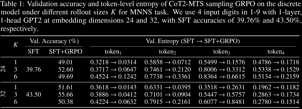
CoT2-MTS improves validation accuracy relative to the discrete baseline. Smaller $K$ values lead to larger reductions in token-level entropies, suggesting it learns to commit to fewer tokens. A curriculum on $K$ may help: start small, and gradually increase.

Appendix C.2 shows that CoT2 with CSFT performs well once the embedding dimension is large, and Dirichlet sampling (rather than MTS) can improve performance even further.

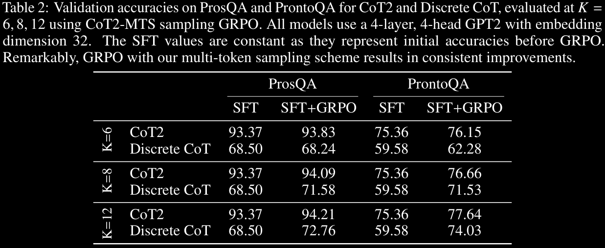
All choices seem to work pretty well, with fairly significant improvements for CoT2 over Discrete CoT. The difference is particularly pronounced in ProsQA, but only minor on ProntoQA.

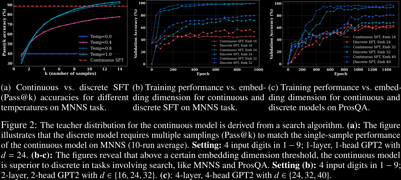
Finally, we display a figure from earlier in the paper. They show that continuous SFT outperforms the discrete baseline once the embedding dimension is high enough, and actually convergence may be faster too; see Figures 2b and 2c. Figure 2a demonstrates that the discrete model requires multiple samples (Pass@k) to approach a single attempt from the CSFT CoT2.

Further results are given in Appendix C of the paper.