Rethinking Thinking Tokens: LLMs as Improvement Operators

• Rethinking Thinking Tokens: LLMs as Improvement Operators
• 2025-10; Madaan, Didolkar, Gururangan, Quan, Silva, Sadakhutdinov, Zaheer, Arora, Goyal

High-Level Summary

• Reframes "thinking" as an improvement operator
• Introduces Parallel-Distill-Refine (PDR):
  1. Generate diverse drafts in parallel (low latency)
  2. Distil into a bounded, textual workspace
  3. Refine current answer based on this workspace
• Workspace is non-persistent; boundedness ensures linear compute
• Primarily measure performance vs sequential budget (proxy for latency)

Elevator Pitch

Training LLMs to reason incentivises them to output their chain of thought (CoT). This allows exploration of different strategies, and backtracking, but comes at a significant computational cost: their CoTs can be very long, inflating the context length by an order of magnitude and more. This is expensive, both in terms of compute and latency, since it is serialised, not parallelised.

Parallel-Distill-Refine (PDR) addresses this by providing a bounded workspace in which the "thinking" occurs. The workspace does not persist between rounds, so the context does not grow. PDR generates drafts in parallel, distils them to the workspace and then refines the current answer based on this workspace.

The authors measure accuracy against sequential budget, a proxy for latency. When no parallelisation is used in the first step, they term it Sequential Refine (SR).

Contributions and Findings:

• a scalable, performant framework for thinking;
• improvement over Long CoT at matched latency;
• certainly a basis for future models and research.

Methodology: LLMs as Improvement Operators

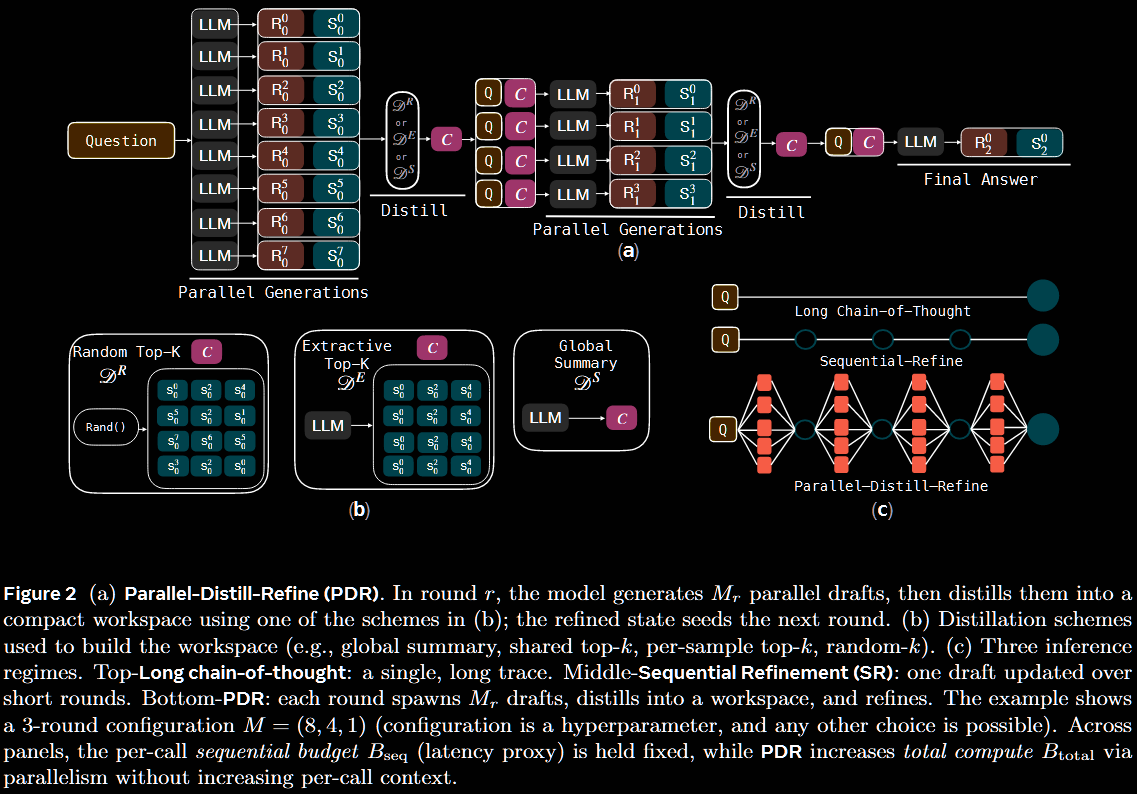
The primary tool introduces is Parallel-Distill-Refine (PDR).

1. Generate $M \ge 1$ diverse drafts in parallel. ($M$ has no effect on latency.)
2. Distil these into a bounded workspace; eg, summarise or pick top-$k$ drafts.
3. Refine answer conditional on this workspace, and repeat.

If no parallelisation is used (ie, $M = 1$), PDR is termed Sequential-Refine (SR).

Problem Setting and Notation

Given a task $x$, the objective is to produce a high-quality final artefact/solution $s_\textsf{final}$ under a given token budget. The (frozen or trainable) LLM, used as an improvement operator, is denoted $\mathcal M_\theta$.

Given current artefact $s_t$ and a textual workspace $C_t$, the model refines: $$s_{t+1} := \mathcal M_\theta(x, s_t, C_t).$$ The workspace $C_t$ is a bounded summary ($|C_t| \le \kappa$) meant to capture agreements, contradictions, intermediate results and goals and the like. The workspace is updated via some distilation operator: $$C_{t+1} := \mathcal D(x, s_{t+1}).$$

Methods are evaluated under two budgets.

• Sequential, $B_\textsf{seq} := \sum_{c \in \mathcal P} (\text{in}_c + \text{out}_c)$:
  • tokens along the accepted path $\mathcal P$ only;
  • a latency proxy, assuming sufficiently parallelisation.
• Total, $B_\textsf{tot} := \sum_{c=1}^C (\text{in}_c + \text{out}_c)$:
  • all calls, including discarded branches;
  • compute/cost proxy.

Here, $c = 1, ..., C$ indexes all model calls, and $\text{in}_c$/$\text{out}_c$ is the input/output tokens for call $c$; $\mathcal P \subseteq \{1, ..., C\}$ is the final accepted path.

Operator Instantiations

A persistent memory is not maintained. Instead, for rounds $r = 1, ..., R$, $M_r$ drafts are sampled in parallel conditioned on the current bounded summary, which resynthesised (distil) a fresh bounded summary: $$\begin{aligned} S^{(r)} &:= \{ s^{(r)}_i := \mathcal M_\theta(x, C^{(r-1)}) \}_{i=1}^{M_r}; \\ C^{(r)} &:= \mathcal D(x, S^{(r)}), \quad C^{(0)} := \varnothing, \quad |C^{(r)}| \le k. \end{aligned}$$ We enforce $M_R = 1$, and it returns $s_\textsf{final}$. To reiterate, the summary is roundwise and non-persistent.

There are multiple ways to construct the roundwise summary.

1. Global summary: produce a single, shared $C^{(r)}$ capturing agreements, contradictions, derived facts, unresolved subgoals, next actions and the like.
2. Top-$k$ evidence: instead of free-form text, select $k$ solutions from $S^{(r)}$ as the workspace itself.
3. Random-$k$ bootstrapped: construct multiple small workspaces by randomly sampling $k$ solutions per generation; different parallel generations get different workspaces.

Operator-Consistent Training

Reasoning models have typically been trained to optimise a single, long CoT trajectory. Using PDR at inference creates a train–test mismatch. This is addressed by using two modes.

1. Standard, long-trace optimisation.
2. Operator rollouts that execute generate → distil → refine under shorter contexts.

The base algorithm is CISPO from MiniMax-M1 (2025/06), which is a GRPO variant. To improve stability, they include an SFT loss: $$J(\theta) := J_\textsf{CISPO}(\theta) + \alpha J_\textsf{SFT}(\theta)$$ where $\alpha := 0.1$ and $$J_\textsf{SFT}(\theta) := \mathbb E_{x \sim \mathcal D} \mathbb E_{o_1, ..., o_G \sim^\textsf{iid} \pi_{\theta_\textsf{old}}(\cdot \mid x)}\biggl[ - \frac1{|\mathcal I^+|} \sum_{i \in \mathcal I^+} \frac1{|o_i|} \sum_{t=1}^{|o_i|} \log \pi_\theta(o_{i, t} \mid x, o_{i, < t}) \biggr].$$ The CISPO objective ensures the RL explores diverse strategies and learns from both successes and failures. The SFT objective adds stability and strongly reinforces correct solutions, but does not learn from mistakes.

To address the train–test mismatch, a data mixture is used: at each update, the mini-batch $\mathcal B$ is split evenly into two sub-batches, $\mathcal B_\textsf{tr}$ and $\mathcal B_\textsf{op}$.

• Training on $\mathcal B_\textsf{tr}$ uses the standard long-CoT framework.
• Training on $\mathcal B_\textsf{op}$ uses PDR with only one round.

The datamix is designed to preserve competence on long traces whilst also teaching the model to reason across short iterations.

Whilst PDR is only trained with $R = 1$ round, we can run $R > 1$ rounds at inference.

Teach someone to fish (R = 1), and they'll be fed for life (R > 1).

Experimental Results

The models gpt-o3-mini and gemini-2.5-flash are evaluated on the AIME '24 & '25 benchmarks. Performance is reported as a function of both the sequential budget $B_\textsf{seq}$ (ie, 'latency') and total budget $B_\textsf{tot}$ (ie, 'cost').

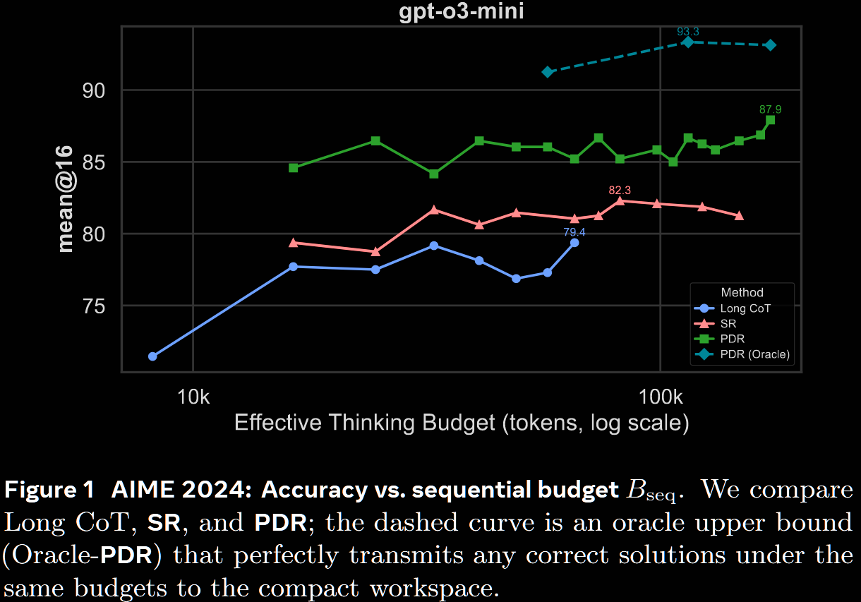
The first figure compares long CoT, PDR & SR at matched sequential budgets on the AIME '24 benchmark.

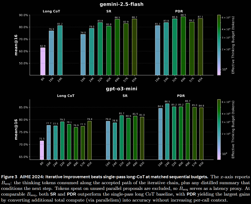
• Gemini 2.5: PDR is slightly more performant than long CoT at 24k, with a larger gap at 16k; SR is worse
• GPT o3: both PDR and SR outperform long CoT at all budgets, with a marked improvement from 77.5% to 86.5% at 24k.

The difference is starker for GPT-o3 than Gemini 2.5, but this may be more a consequence of its lower baseline vs Gemini 2.5.

The next figure uses only Gemini 2.5, but also compares total budget.

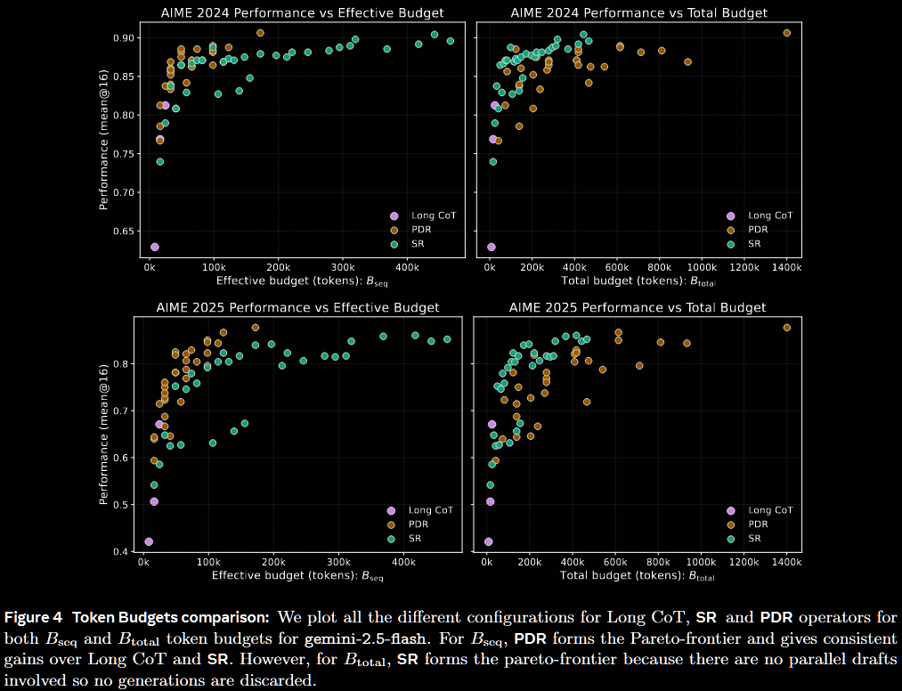
• Latency:
  • PDR outperforms long CoT, and exploits parallelisation to fill the Pareto frontier
  • whilst SR achieves competitive performance, its sequential nature leads to large latency
• Cost:
  • SR can outperform long CoT, but possibly at an increased cost
  • PDR performs well, but its parallelisation is compute-hungry
  • unfortunately, the long CoT runs have too low a budget to make a firm conclusion

Alas, the lack of a log scale on the horizontal axis makes the visualisation rather cluttered.

Further experiments are given in the paper, all motivated by four research questions/objectives.

1. Can short-context iterations outperform long traces?
2. Figure out the best distillation strategy.
3. Identify the effect of verification ability of a given model.
4. Can operator-consistent training shift the Pareto frontier.

Conclusion

The bounded-workspace approach certainly offers improved latency at high token counts, since the (sequential) compute is linear, not quadratic. Its parallelisation also appears to offer performance improvements, albeit potentially at a high total cost.