Reasoning with Sampling: Your Base Model is Smarter Than You Think

• Reasoning with Sampling: Your Base Model is Smarter Than You Think
• 2025-10; Karan, Du
• GitHub: https://github.com/aakaran/reasoning-with-sampling/tree/main

High-Level Summary

• Capability vs Sampling:
  • There is significant debate/interest in whether RL post-training develops new capabilities or just sharpens sampling
  • If it's the latter, perhaps the distribution can be sharpened without any post-training
• Paper's contribution:
  • Uses a Markov chain to sample from sharpened power distributions ($p^\alpha$ instead of $p$, for some $\alpha \ge 1$)
  • Find substantial gains over base model and comparable with RL-post-trained versions
  • No training, datasets, verifiers or the like are needed

Elevator Pitch

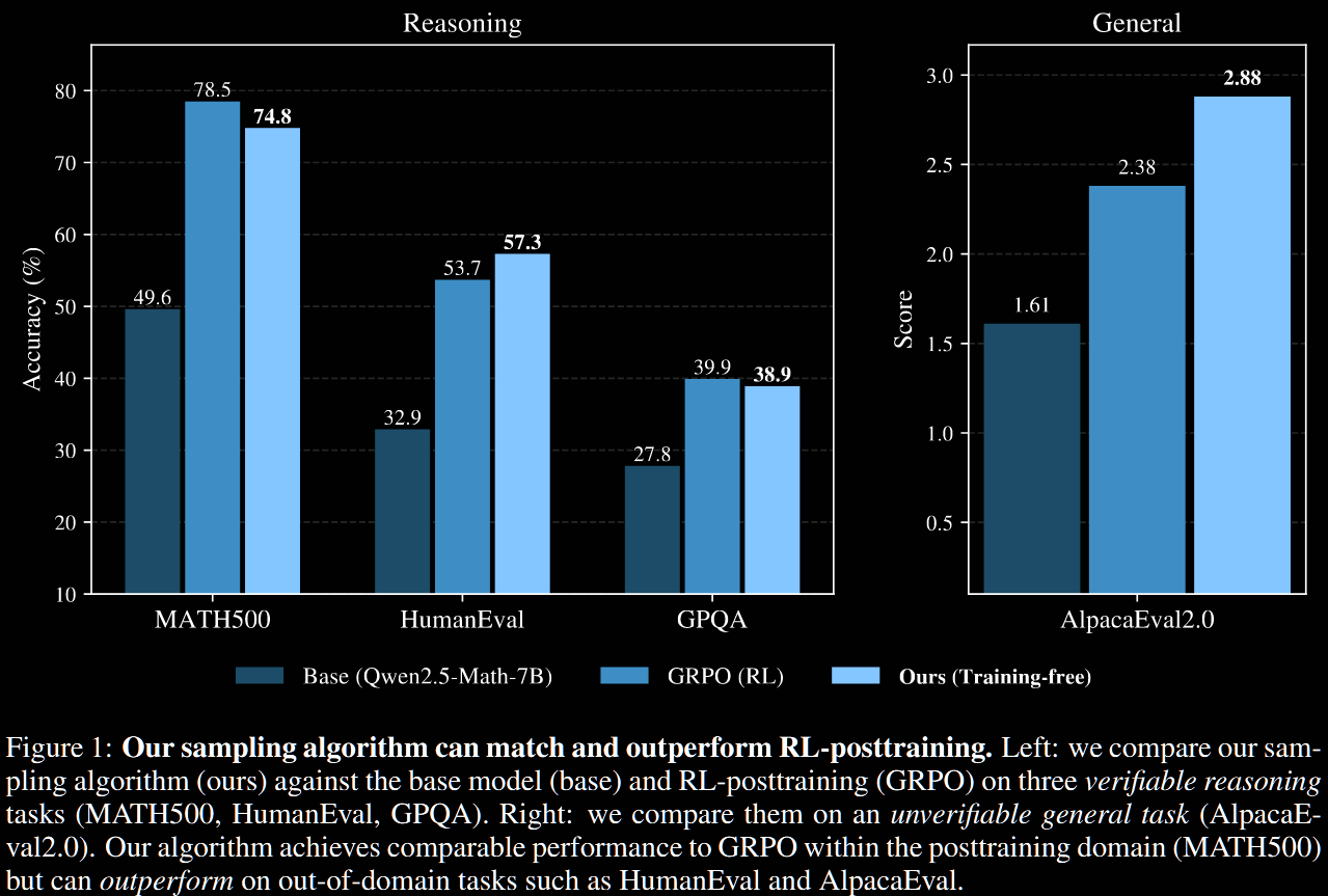
Post-training an LLM with RL often provides impressive improvements for pass@1, but pass@k decays for large $k$. This raises the question, "Does RL develop new capabilities, or simply sharpen the distribution?" Eg, it may collapse to high-reward modes.

The current work achieves similar pass@1 performance increase by pure sampling, without RL. Moreover, pass@k remains competitive with the base even for $k$ up to $16$.

Training LLMs to reason incentivises them to output their chain of thought (CoT). This allows exploration of different strategies, and backtracking, but comes at a significant computational cost: their CoTs can be very long, inflating the context length by an order of magnitude and more. This is expensive, both in terms of compute and latency, since it is serialised, not parallelised.

Contributions and Findings:

• sharpening distributions can match RL post-training
• sharpening can require expensive test-time compute
• performance boost appears to persist for larger pass@k

Methodology for Sharpening

Sharpening a distribution corresponds to reweighting it so that high-likelihood regions becomes even higher, whilst low-likelihood become even lower.

Power Distributions

The authors utilise power distributions:

given a distribution $p$ and real $\alpha$, the power distribution $p^\alpha$ is defined such that $p^\alpha(x) \propto p(x)^\alpha$ for all $x$.

Importantly, this is different to changing the temperature of the LLM sampler: $$\begin{aligned} p_{\textsf{pow}(\alpha)}(x_t \mid x_{< t}) &\textstyle \propto \sum_{x_{> t}} p(x_{< t}, x_t, x_{> t})^\alpha, \\ p_{\textsf{temp}(\alpha)}(x_t \mid x_{< t}) &\textstyle \propto \bigl( \sum_{x_{> t}} p(x_{< t}, x_t, x_{> t}) \bigr)^\alpha, \end{aligned}$$ where $p_{\textsf{pow}(\alpha)} = p^\alpha$ is the $\alpha$-power distribution and /$p_{\textsf{temp}(\alpha)}$ is the $1/1\alpha$-temperature distribution.

Intuitively, low-temperature sampling affects only the current token: it does not account for the likelihood of "future paths". Conversely, the power distribution up-weights the entire path. Naturally, sampling from $p^\alpha$ exactly is computationally intractable—even calculating the normalising constant is. Instead, a Metropolis–Hastings algorithm is used.

Metropolis–Hastings

The authors use a standard Metropolis–Hastings (MH) algorithm. This draws approximate samples from a target distribution $\pi$ given only a proposal distribution $q$. It is iterative:

• if $x_t = x$, draw $y \sim q(\cdot \mid x)$;
• accept $y$, setting $x_{t+1} := y$, with probability $A(x, y)$ where $$A(x, y) := \min\biggl\{ 1, \: \frac{ q(y \mid x) \pi(x) }{ q(x \mid y) \pi(y) } \biggr\};$$
• otherwise, reject $y$, setting $x_{t+1} := x$.

It is well known that the associated Markov chain converges to $\pi$ under mild conditions on $q$.

Being able to evaluate $\pi(\cdot)$ is not necessary, only calculating ratios is; in particular, an unnormalised version can be used instead. Practically, both $q(x \mid y)$ and $q(y \mid x)$ should be easily computable—or, at least, their ratio.

The target distribution in the current set-up is $\pi := p^\alpha$; the choice of $q$ is open. The following process is used:

given sequence $x = (x_1, ..., x_T)$, choose $L \sim \operatorname{Unif}(\{1, ..., T\})$ and resample the sequence starting at index $L$ using an LLM-proposal distribution $p_\textsf{prop}$.

The transition probabilities $q(y \mid x)$ and $q(x \mid y)$ are then simple to calculate. The flexibility of MH means that $p_\textsf{prop}$ can be any LLM with any sampling strategy.

Power Sampling with MH

The Markov chain does converge to $\pi = p^\alpha$, but its mixing time—ie, the number of steps needed until its law is close to its target measure $\pi = p^\alpha$—may be large. The space is high dimensional, since we allow long sequences, so the mixing time could even be exponential in $T$. For this reason, the proposed algorithm proceeds in blocks.

Fix a block size $B$ and proposal LLM $p_\textsf{prop}$. Let $\pi_k$ be the distribution given by $\pi_k(x_{1:kB}) \propto p(x_{1:kB})^\alpha$, and consider the sequence of distributions $$\varnothing \to \pi_1 \to \pi_2 \to \cdots \to \pi_T = p.$$ We proceed inductively along $k$.

To sample $x_{1:kB} \sim \pi_k$:

• initiate a MH algorithm by sampling $x_{1:(k-1)B} \sim \pi_{k-1}$ (by induction);
• sample the next $B$ tokens $x_{(k-1)B+1:kB}$ with $p_\textsf{prop}$;
• subsequence MH proposals resample from $L \sim \operatorname{Unif}(\{1, ..., kB\})$;
• this is repeated for $N$ iterations.

The scaling is quantified by estimating the average number of tokens generated by this algorithm. Each candidate generation step when sampling $\pi_k$ resamples an average of $\tfrac12 k B$ tokens (approximately), and this is repeated $N$ times. Summing over $k$ gives $$\textstyle \mathbb E_\text{tokens} \approx N \sum_{k=1}^{T/B} \tfrac12 k B \approx \tfrac14 T^2 N / B.$$ There is a tradeoff between the block size $B$ and the number of Markov-chain steps $N$.

Author note. Compute grows quadratically in the sequence length. So, the number of tokens used is not necessarily the most interesting proxy. If computing token in position $t$ takes $t$ units of compute, the expected amount of compute per step in iteration $k$ is $$\textstyle \tfrac1{kB} \sum_{\ell=1}^{kB} \sum_{t=\ell}^{kB} t \approx \tfrac1{kB} \sum_{\ell=1}^{kB} (\tfrac12(kB)^2 - \tfrac12 \ell^2) \approx \cdots \approx \tfrac13 (k B)^3.$$ Multiplying this by $N$ and summing over $k$ gives $$\textstyle \mathbb E_\textsf{compute} \approx N \sum_{k=1}^{T/B} \tfrac13 (k B)^2 \approx \tfrac19 T^2 N / B.$$ Conversely, the compute for direct, long-CoT sampling is $$\textstyle \sum_{t=1}^T t \approx \tfrac12 T^2.$$

The Markov chain doesn't necessarily need to be that well mixed. Empirically, the authors find a value for $B$ that makes the algorithm work well for relatively small values of $N$; see the next section for details.

Author note. There appears to be some nested structure: to sample $x_{0:kB} \sim \pi_k$, first sample from $x_{0:(k-1)B} \sim \pi_{k-1}$ and fix it; then, sample $x_{(k-1)B+1:kB}$ conditionally on $x_{0:(k-1)B}$. This could allow the MH proposal to resample from $L$ uniformly from $\{(k-1)B + 1, ..., kB\} \subseteq \{1, ..., kB\}$. This would reduce the average number of resampled tokens from $\tfrac12 kB$ to $\tfrac12 B$, resulting in $$\textstyle \mathbb E_\textsf{tokens} = N \sum_{k=1}^{T/B} \tfrac12 B = \tfrac12 T N.$$ It's possible that a larger $N$ would be required, or potentially one that depends on $k$ with $N_k \to \infty$ as $k \to \infty$.

Experiments

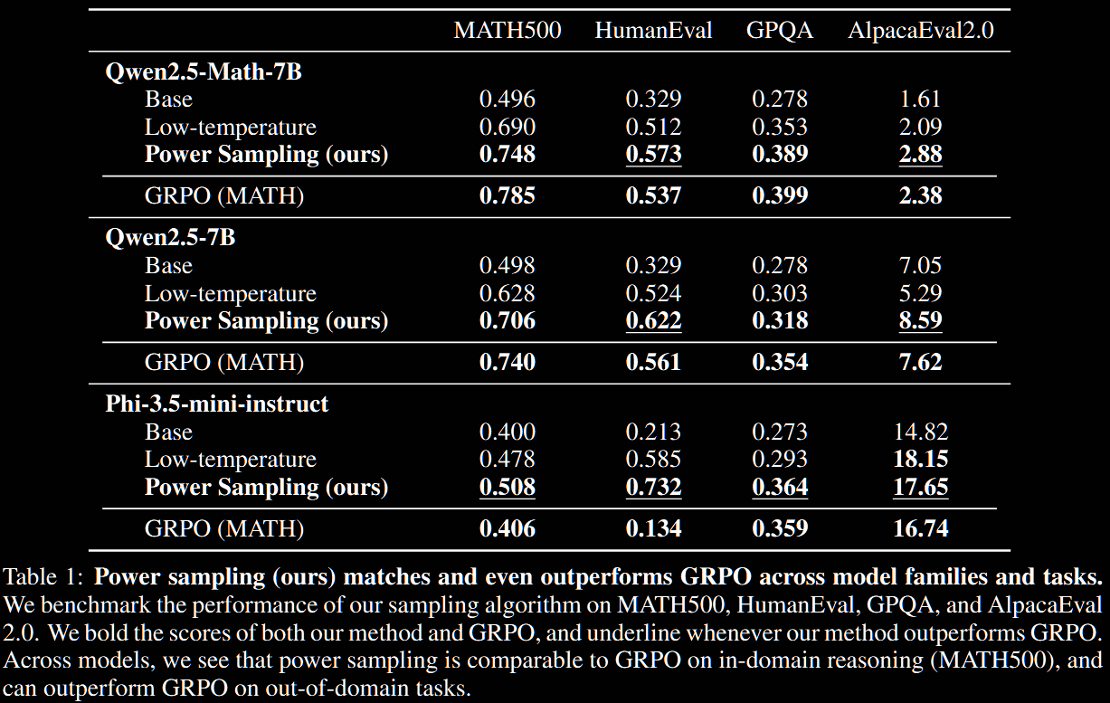
A standard suite of reasoning benchmarks is used: MATH500, HumanEval, GPQA-Diamond, AlpacaEval-2.0. Base models Qwen2.5-Math-7B, Qwen2.5-7B and Phi-3.5-mini-instruct are used.

Author note. The Qwen models may have been exposed to certain benchmarks during training. This could make them more amenable to sharpening methods—whether power-distribution sharpening or RL.

The following parameters are used.

• Maximum length $T_\textsf{max} := 3072$; early termination is possible with EOS token
• Split into 16 blocks, so $B := T_\textsf{max} / 16 = 3072 / 16 = 192$, with $N = 10$ steps
• Power-exponent $\alpha = 4.0$ with proposal LLM the base LLM with temperature $\tau = 1/\alpha = 0.25$
• For AlpacaEval 2.0, a slightly higher proposal temperature of $\tau = 0.5$ improves performance

Main Results

The sharpened version achieves significant, "near-universal" boosts (as the paper puts it) in single-shot accuracies and scores across different reasoning and evaluation task versus the base algorithm. This includes +51.9% on Human Eval with Phi-3.5-mini and +25.2% on MATH500 with Qwen2.5-Math-7B. In particular, on MATH500, which is in-domain for RL post-training, power sampling achieves accuracies on par with those obtained by GRPO.

A defining, and arguably negative, feature of RL post-training is the long reasoning traces. On MATH500, Qwen2.5-Math-7B averages 600 tokens, whilst its GRPO version averages 671; surprisingly, power-sampling averages a similar 679 tokens without explicit encouragement.

Sampling vs Capability

The likelihoods/confidences of GRPO are more peaked and concentrated than for power sampling; see Figure 4, not repeated here. This suggests a collapse in diversity for GRPO not present in power sampling.

To quantify this, various pass@k metrics are plotted; Qwen2.5-Math-7B is used as the base model in the four plots below.

 

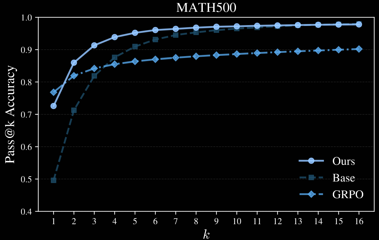
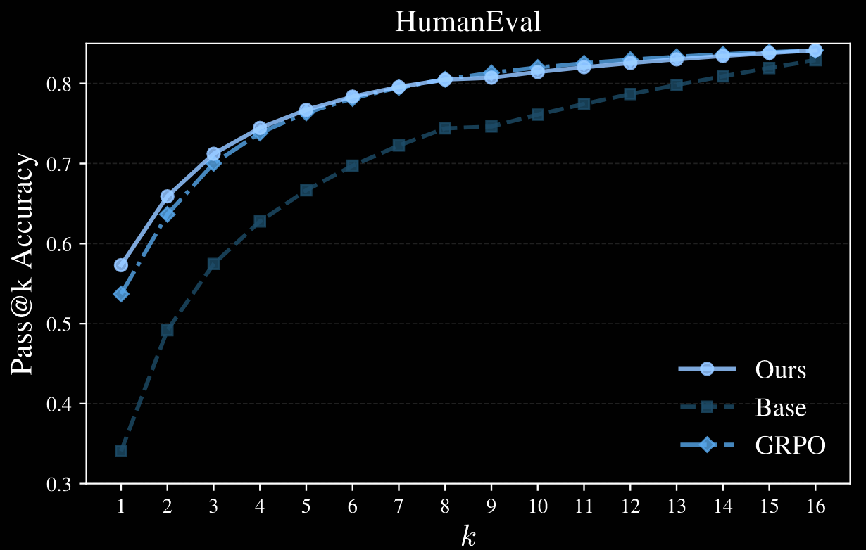
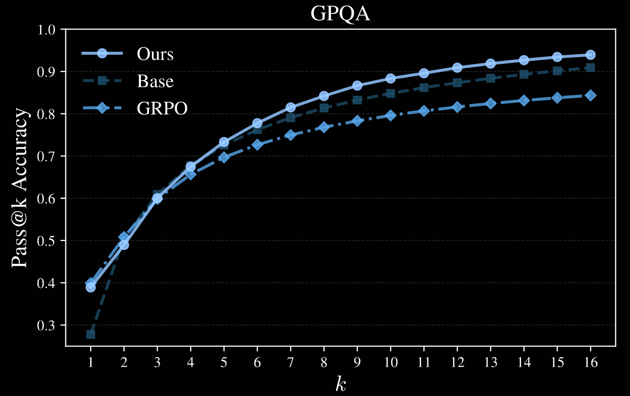
Author note. It's a shame the authors only went up to $k = 16$. This appears to be sufficient for MATH500, but higher values would certainly be interesting for HumanEval and GPQA; AlpacaEval is not plotted.

Exponent and Mixing-Time Hyperparameters

A light ablation on $\alpha$ and $N = N_\text{MCMC}$ is given.

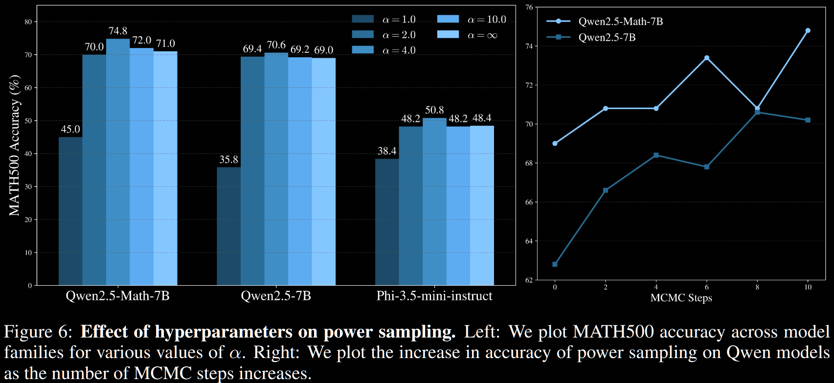
It is not plotted, but the authors claim that accuracy remained roughly stable for $N \ge 10$.

Test-Time Scaling

Using MH to approximate the power distribution at test time incurs test-time scaling costs vs standard, long-CoT inference:

• roughly $\tfrac14 T N / B$ times as many tokens;
• roughly $\tfrac29 T N / B$ times as much compute.

These factors are pretty close. Taking MATH500 on Qwen2.5-Math-7B as an example on which the average length is $T = 679$ tokens, with $B = 192$ and $N = 10$, $$\tfrac14 T N / B \approx 8.8 \quad\textsf{and}\quad \tfrac29 T N / B \approx 7.9.$$ In other words, about an extra order of magnitude of compute/tokens is required.

GRPO training typically uses 8–16 rollouts per sample, which is not so dissimilar. On the one hand, that may be run over many epochs, on larger datasets, requiring much more compute. On the other, once it's done, it's done, whilst power-sampling requires this every time it's used: it's a latency cost.

Conclusion

The paper makes a strong case for sharpening distributions. They nearly match performance on RL-post-trained systems for pass@1, but appear to avoid model collapse issues highlighted by deterioration in RL's pass@k performance for large $k$.

It would be very interesting to investigate further sampling methods to really unlock base models' inherent capability.

Of course, the order-of-magnitude token/compute cost at inference is not ideal. More efficient methods would certainly be desirable.