Hierarchical Reasoning Model

• Hierarchical Reasoning Model
• 2025-06; Wang, Li, Sun, Chen, Liu, Wu, Lu, Song, Yadkori

High-Level Summary

• Introduces Hierarchical Reasoning Model (HRM), a new small model
• A recurrent architecture modelled on hierarchical and multi-timescale processing in human brains
• Attains significant computational depth whilst maintaining both training stability and efficiency
• Small model: only 27M parameters
• operators without pre-training: task-specific training

Elevator Pitch

Current LLMs primarily employ CoT techniques to reason. These suffer from computational challenges, including requiring extensive data. Also, are they really reasoning? Or, are they recalling reasoning they've seen? Their struggles on novel tasks, such as in ARC, hint at the latter.

Inspired by hierarchical processing and temporal separation in the human brain, HRM has two interdependent recurrent modules:

• a high-level module responsible for slow, abstract planning;
• a low-level module handling rapid, detailed computations.

The model operates without pre-training of CoT data. Rather, training data is required for the task at hand—eg, ARC-AGI-2 or Maze-Hard. This checkpoint is not saved for future tasks: the model is randomly initialised for each task.

HRM outperforms much larger models with significantly longer context windows on ARC, and achieves excellent performance on complex tasks, such as Sudoku or optimal path finding in large mazes, where CoT models fail completely.

Detailed Motivation

LLMs largely rely on CoT prompting for reasoning. CoT externalises reasoning into language, breaking down complex tasks into simpler, intermediate steps. Such a process lacks robustness and is tethered to linguistic patterns; it requites significant training data and generates many tokens, resulting in large computational cost. Humans certain don't reason this way.

Enter latent reasoning: the model internalises computations. This aligns with the understanding that language is tool for communication, not the substrate of thought itself. Latent reasoning is fundamentally constrained by a model's effective computational depth. Naively stacking layers leads to vanishing gradients. Recurrent architectures often suffer from early convergences—internal state stabilises, and further calculations are useless, and rely on computationally expensive backprop through time (BPTT) training.

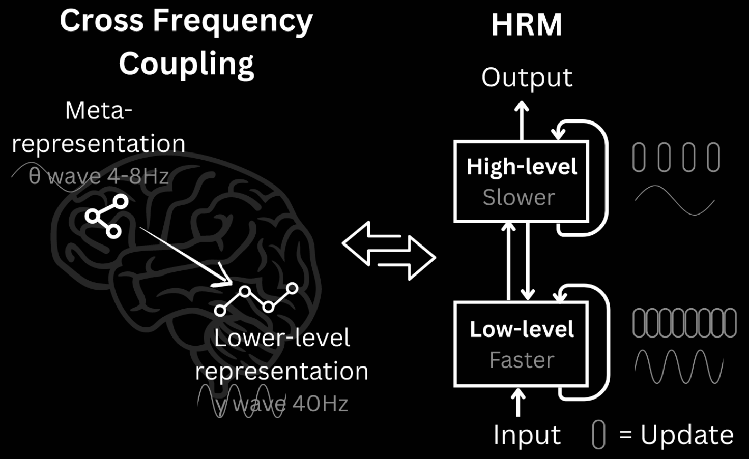
The human brain organises computation hierarchically across different regions, operating at different timescales. Slow, higher-level areas guide fast, lower-level circuits via recurrent feedback loops. This increases the effective depth, without the cost of BPTT.

HRM is designed to significantly increase the effective computational depth. It features two coupled recurrent modules:

• high-level for slow, abstract reasoning;
• low-level for fast, detailed computations.

The slow module (H) advances only after the fast one (L) has reached a local equilibrium, at which point it is reset. This avoids the early convergence of standard recurrent models.

Further, a one-step gradient approximation for training HRM is used, maintaining $O(1)$ memory footprint (vs $O(T)$ for $T$ timesteps in BPTT), applying backprop in a single step at the equilibrium point.

HRM

The HRM consists of four learnable components:

• an input network $f_I(\cdot; \theta_I)$;
• a low-level recurrent module $f_L(\cdot; \theta_L)$;
• a high-level recurrent module $f_H(\cdot; \theta_H)$;
• an output network $f_O(\cdot; \theta_O)$.

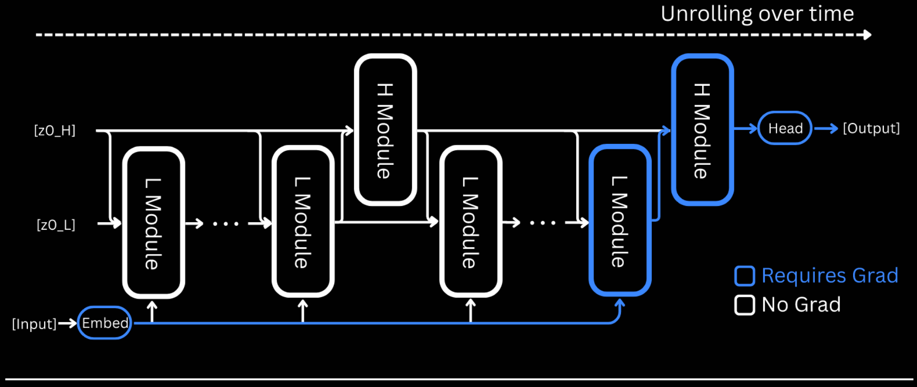
The models' dynamics unfold over $N$ high-level cycles, each consisting of $T$ low-level steps. The modules $f_{L/H}$ each keep a hidden state $z_{L/H}$.

First, the framework is outlined, including some brief architectural details, then the training recipe explained. The section closes with detailed pseudocode for training.

Framework

The HRM maps an input vector $x$ to an output prediction vector $\hat y$ as follows.

1. Convert the input $x$ into a working representation $\tilde x$: $$\tilde x := f_I(x; \theta_I).$$

2. At each timestep $i = 1, ..., NT$, the L module updates its state and the H module updates only if a multiple of $T$ as follows: $$\begin{aligned} z_L^i &:= f_L(z_L^{i-1}, z_H^{i-1}, \tilde x; \theta_L); \\ z_H^i &:= \begin{cases} z_H^{i-1} &\text{if}\quad i \not\equiv 0 \text{ mod } T, \\ f_H(z_H^{i-1}, z_L^i; \theta_H) &\text{if}\quad i \equiv 0 \text{ mod } T. \end{cases} \end{aligned}$$ Alternatively, one could only define the H state every T updates—ie, the 'real' updates, $z_H^0, z_H^T, ..., z_H^{NT}$. The HRM paper mixes the two versions, unfortunately.

3. After $N$ full cycles, a prediction $\hat y$ is extracted from the hidden state of the H module: $$\hat y := f_O(z_H^{NT}; \theta_O).$$

This entire three-step process represents a single forward pass. A halting mechanism (discussed below) determines whether the model should terminate, in which case $\hat y$ is output, or continue with an additional forward pass.

Whilst convergence is crucial for recurrent networks, it also limits their effective depth—iterations the (almost) convergence point add little value. HRM addresses this by alternating between L-convergence and H-iteration: a single H update establishes a fresh context for the L module, 'restarting' its convergence.

HRM uses a sequence-to-sequences architecture: both the input $x = (x_1, ..., x_\ell)$ and output $\hat y = (\hat y_1, ..., \hat y_{\ell'})$ are represented as sequences.

• The embedding layer $f_I$ converts discrete tokens into vector representations.
• The output head $f_O$, given by $f_O(z; \theta_O) = \operatorname{softmax}(\theta_O z)$, transforms hidden states into token probability distributions $\hat y$.
• Both low- and high-level recurrent modules $f_L$ and $f_H$, respectively, are encoder-only Transformer blocks, with identical architectures and dimensions.

Training Recipe

The training recipe consists of three main aspects. These are outlined below; detailed descriptions are given in collapsible sections, but may be skipped.

1. Deep Supervision. Given a data sample $(x, y)$, multiple forward passes of HRM are run. Let $z^m := (z^{m N T}_H, z^{m N T}_L)$ and $\theta^{m-1}$ denote the hidden state and parameters, respectively, at the end of segment $m$.

   1. $(z^m, \hat y^m) := \mathsf{HRM}(z^{m-1}, x; \theta^{m-1})$.
   2. $L^m := \mathsf{Loss}(\hat y^m, y)$.
   3. $\theta^m := \mathsf{OptimiserStep}(\theta^{m-1}, \nabla_\theta L^m)$.

2. Adaptive Computation Time (ACT): halting strategy and loss function. With deep supervision, each mini-batch is used for up to $M_\textsf{max} = 16$ steps. A halting strategy, for early stopping during training, is learned through a Q-learning objective. It greatly diminishes the time spent per example on average, at least for the Sudoku-Extreme dataset (only reported). It does, however, require an extra forward pass with the current parameters to determine if halting now is preferable to later.

   Adaptive Computational Time (ACT): Halting strategy and loss function.

   The adaptive halting strategy uses Q-learning to adaptively determine the number of segments (forward passes). A Q-head uses the final state of the H module to predict the Q-values: $$\hat Q^m = (\hat Q^m_\textsf{half}, \hat Q^m_\textsf{cont}) = \operatorname{sigmoid}(\theta_Q^\top z_H^{m N T}).$$ The half/cont(inue) action is chosen using a randomised strategy.

   • Let $M_\textsf{max}$ denote the maximum number of segments (a fixed hyperparameter).
   • Let $M_\textsf{min} := 1 + \operatorname{Bern}(\varepsilon) \operatorname{Unif}(\{0, ..., M_\textsf{max} - 1\})$ denote the minimum number of segments.
   • The halt action is selected if $m \ge M_\textsf{min}$ and either $m \ge M_\textsf{max}$ or $\hat Q_\textsf{half} > \hat Q_\textsf{cont}$.

   The Q-head is updated through a Q-learning algorithm. The state of its episodic Markov decision process (MDP) at segment $m$ is $\tilde z^m := z_H^{m N T}$ and the action space is $\{\textsf{halt}, \textsf{cont}\}$.

   • Choosing $\textsf{halt}$ terminates the episode and returns the binary reward indicating correctness: $\mathbf 1\{ \hat y^m = y \}$.
   • Choosing $\textsf{cont}$ yields a reward of $0$ and the state transitions to $\tilde z^{m+1}$.

   The Bellman equations define the optimum: $$\begin{aligned} Q^\star_\textsf{halt}(\tilde z) &= \mathbb E[ \mathbf 1\{ \hat y^m = y \} ]; \\ Q^\star_\textsf{cont}(\tilde z) &= \mathbb E[ \max\{Q^\star_\textsf{halt}(\tilde z), Q^\star_\textsf{cont}(\tilde z)\} ]. \end{aligned}$$

   The optimum $Q^\star_\textsf{halt/cont}(\tilde z)$ is interpreted as the probability of being correct given halting/continuing, given that the current state is $\tilde z$.

   Thus, the Q-learning targets $\hat G^m = (\hat G^m_\textsf{halt}, \hat G^m_\textsf{cont})$ for the two actions are given as follows: $$\begin{aligned} \hat G^m_\textsf{halt} &:= \mathbf 1\{ \hat y^m = y \}; \\ \hat G^m_\textsf{cont} &:= \begin{cases} \hat Q^{m+1}_\textsf{halt} &\text{if}\quad m \ge M_\textsf{max}, \\ \max\{ \hat Q^{m+1}_\textsf{halt}, \hat Q^{m+1}_\textsf{cont} \} &\text{otherwise} \end{cases} \end{aligned}$$ This last expression corresponds to the probability of being correct given continuing at step $m$: either stop at step $m+1$ ($\hat G^{m+1}_\textsf{halt}$) or continue beyond ($\hat G^{m+1}_\textsf{cont}$).

   We can now define our loss function: [ \mathcal L^m = \textsf{Loss}(\hat y^m, y)

   • \textsf{BinaryCrossEntropy}(\hat Q^m, \hat G^m). ] Minimising this enables both accurate predictions and sensible stopping decisions.

3. One-Step Gradient Approximation. Assuming that $(z_L, z_H)$ reaches a fixed-point $(z_L^\star, z_H^\star)$ through recursion, the implicit function theorem with one-step gradient approximation allows approximation of the gradient by backproping only the last step.

   The legitimacy of the application to this set-up, with so fewer steps in the iteration, is questionable.

   Theoretical foundation for one-step gradient approximation.

   The one-step gradient approximation is based on deep equilibrium models, which employ the implicit function theorem to bypass BPTT.

   In idealised HRM behaviour, during the $k$-th high-level cycle, in state $z_H^{k-1}$, the L module iterates its state $z_L$ to a local fixed point $z_L^\star$. This can be expressed in the form $$z_L^\star = f_L(z_L^\star, z_H^{k-1}, \tilde x; \theta_L),$$ where $\tilde x = f_I(x; \theta_I)$. The H module then performs a single update using this converged state: $$z_H^k = f_H(z_H^{k-1}, z_L^\star; \theta_H),$$ In other words, $$z_H^k = f(z_H^{k-1}, \tilde x; \theta)$$ for some $f$, where $\theta = (\theta_I, \theta_L, \theta_H)$. Its fixed point $z_H^\star = z_H^\star(\theta, \tilde x)$ satisfies $$z_H^\star = f(z_H^\star; \theta).$$ The implicit function theorem allows calculation of the exact gradient of the fixed point $z_H^\star$ wrt $\theta$ through the Jacobian $J_F(z_H) := \frac{\partial F}{\partial z_H}$: $$\frac{\partial z_H^\star}{\partial \theta} = \bigl( I - J_F(z_H^\star) \bigr)^{-1} \cdot \frac{\partial F}{\partial \theta} \biggr|_{z_H = z_H^\star}.$$

   Unfortunately, evaluating and inverting $I - J_F(z_H)$ is prohibitively expensive. But, for $z_H$ in a neighbourhood of the fixed point, $J_F(z_H) \approx 0$. This leads to $$\frac{\partial z_H^\star}{\partial \theta_H} \approx \frac{\partial f_H}{\partial \theta_H}, \quad \frac{\partial z_H^\star}{\partial \theta_L} \approx \frac{\partial f_H}{\partial z_L^\star} \cdot \frac{\partial z_L^\star}{\partial \theta_L} \quad\textsf{and}\quad \frac{\partial z_H^\star}{\partial \theta_I} \approx \frac{\partial f_H}{\partial z_L^\star} \cdot \frac{\partial z_L^\star}{\partial \theta_I}.$$ The gradients of the low-level fixed point $z_L^\star$ can be approximated similarly: $$\frac{\partial z_L^\star}{\partial \theta_L} \approx \frac{\partial f_L}{\partial \theta_L} \quad\textsf{and}\quad \frac{\partial z_L^\star}{\partial \theta_I} \approx \frac{\partial f_L}{\partial \theta_I}.$$ Plugging these into the previous display gives the final approximated gradients: $$\frac{\partial z_H^\star}{\partial \theta_H} \approx \frac{\partial f_H}{\partial \theta_H}, \quad \frac{\partial z_H^\star}{\partial \theta_L} \approx \frac{\partial f_H}{\partial z_L^\star} \cdot \frac{\partial f_L}{\partial \theta_L} \quad\textsf{and}\quad \frac{\partial z_H^\star}{\partial \theta_I} \approx \frac{\partial f_H}{\partial z_L^\star} \cdot \frac{\partial f_L}{\partial \theta_I};$$ these depend only on the functions $f_{H/L/I}$.

Pseudocode

# HRM forward pass
def hrm(z, x_, N=2, T=2):
    zH, zL = z

    # iterate modules without gradient
    with torch.no_grad():
        # update L-level module
        for i in range(N * T - 2):
            zL = L_net(zL, zH, x_)
            # update H-level module
            if (i + 1) % T == 0:
                zH = H_net(zH, zL)
    
    # last iteration with gradient
    zL = L_net(zL, zH, x_)
    zH = H_net(zH, zL)
    return (zH, zL), output_head(zH), q_head(zH)

# Adaptive Computational Time
class ACT:
    # parameters
    def __init__(self, M_max, eps=0.1):
        self.M_max = M_max
        self.M_min = 1 + bern(eps) * unif([0, ..., M_max - 1])
    
    # when to halt
    def ACT_halt(self, q, y_hat, y_true):
        target_halt = (y_hat == y_true)
        loss = 0.5 * binary_cross_entropy(q["halt"], target_halt)
        return loss

    # when to continue
    def ACT_cont(q, last_step: bool):
        if last_step:
            target_cont = q["halt"]
        else:
            target_cont = max(q["halt"], q["cont"])
        loss = 0.5 * binary_cross_entropy(q["cont"], target_cont)
    return loss

# Deep supervision
for x_input, y_true in train_dataloader:
    # Prepare inputs
    x_ = input_embeddings(x_input)
    z = z_init
    act = ACT(M_max=16)

    # Multiple forward passes
    for _ in range(act.M_max):
        # HRM forward pass
        z, y_hat, q = hrm(z, x_)
        
        # two-part loss
        loss_ce = softmax_cross_entropy(y_hat, y_true)
        _, _, q_next = hrm(z, x)  # extra forward pass
        loss_act = act.halt(q_next, y_hat, y_true)
        loss = loss_ce + loss_act

        # Update gradients and optimiser
        z = z.detatch()
        loss.backward()
        opt.step()
        opt.zero_grad()

        # early stopping
        if q["halt"] > q["cont"]:
            break

Results

Despite the impressive results, with such a small model, the results section is actually somewhat sparse.

Benchmarks

Three different types of tasks are considered: ARC-AGI, Sudoku and (finding the optimal path in) Mazes. For all benchmarks, HRM models were randomly initialised and trained in the sequence-to-sequence set-up, using the input--output pairs:

• the input and output grids given in ARC-AGI;
• the initial and completed Sudokus;
• the initial maze and the one augmented with the optimal path.

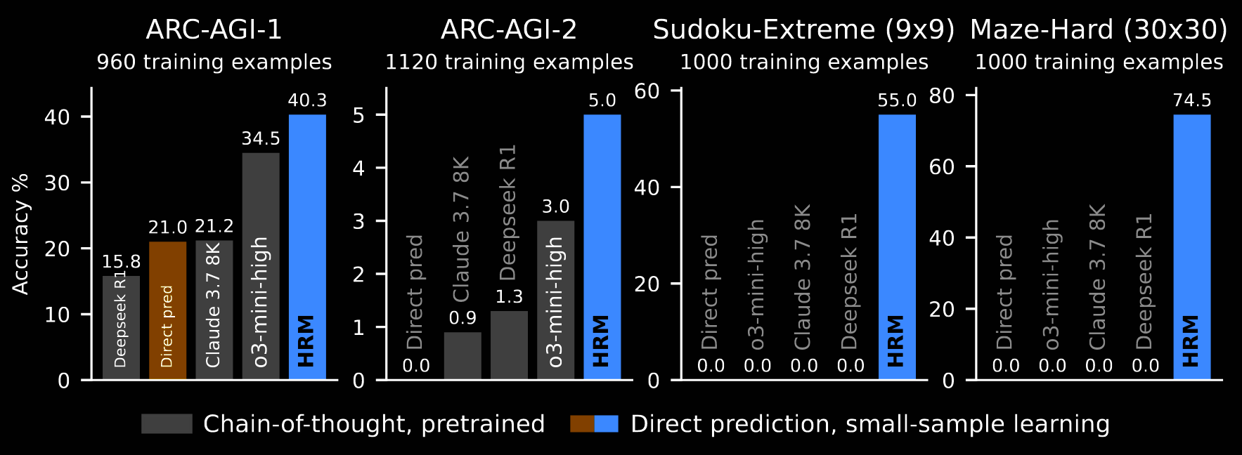
The resulting performance is shown in the previous figure, repeated here. These results are attained with just ~1000 training examples per task, and without pre-training or CoT labels. Various augmentations are implemented for ARC-AGI and Sudoku, but not for the mazes.

The baselines are grouped based on whether they are pre-trained and use CoT (o3-mini-high, Claude 3.7 8K and Deepseek R1) or neither. The "direct pred[iction]" baseline retrains the exact training set-up of HRM, but swaps in a Transformer architecture—eight layers, identical in size to HRM.

• ARC-AGI. HRM outperforms all the LLMs. On ARC-AGI-1, even "direct pred[iction]" outperforms Deepseek R1 and matches the performance of a domain-specific network, carefully designed for learning the ARC-AGI task from scratch, without pre-training.

• Sudoku and Maze. HRM significantly outperforms the baselines here. The benchmarks require lengthy reasoning traces, without much complexity—each step is simple, but there are many of them—making them particularly ill-suited to LLMs.

Data Usage and Augmentation

Data augmentation is relied heavily on for ARC-AGI and Sudoku; it is not used for mazes.

For ARC-AGI, the training dataset starts with all demonstration/example and test/problem input–output pairs from the training set and all demonstration/example pairs from the evaluation set. The test/problem pairs from the evaluation set are saved for test time. The dataset is augmented (eg, colour permutations, rotations, etc). Each pair is prepended with a learnable special token representing its task id.

At test time, for each test/problem pair in the evaluation set, 1000 augmented variants are generated and solved; the inverse augmentation is applied to obtain a prediction. The two most popular predictions are chosen as the final outputs.

To emphasise, the training set is a flattened collection of simple input—output pairs, augmented with the task id. They are not batched by task id. There is no, "Here are X example input–output pairs of grids. The problem is to find the (hidden) output grid corresponding to [this] input grid."

For Sudoku, band and digit permutations are applied. There is no concept of a task to which multiple datapoints belong.

Visualisation

HRM performs well on complex reasoning tasks, raising a question:

"What underlying reasoning algorithm does the HRM neural network actually implement?"

The intermediate stages are visualised. At each timestep $i$, a preliminary forward pass through the H module is performed, then fed through the decoder: $$\tilde z^i := f_H(z_H^i, z_L^i; \theta_H), \quad \tilde y^i := f_O(\tilde z^i; \theta_O).$$ The (intermediate) prediction $\tilde y^i$ is visualised in the figure below; its caption explains what is going on.

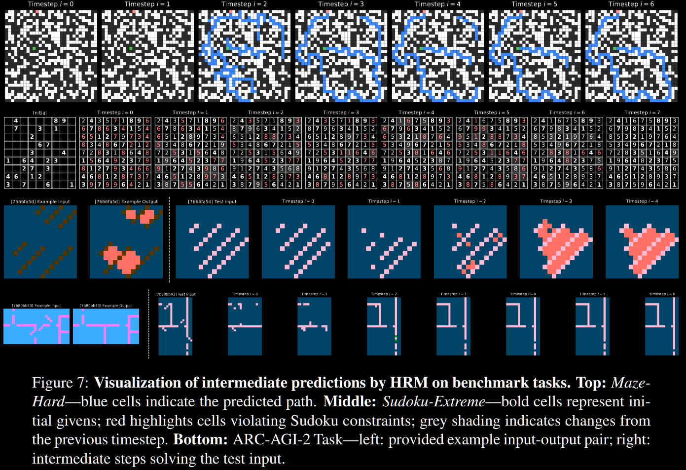
• In the Maze task, HRM appears to explore several poential paths simultaneously, subsequently eliminating blocked/inefficient ones.
• In Sudoku, the strategy resembles a depth-first search, exploring potential solutions and backtracking when it hits dead ends.
• It approaches ARC differently, making incremental adjustments to the grid, iteratively improving until the solution, rather than trying and backtracking. That said, it only solved 5% of ARC-AGI-2, so possibly this is a bad choice.

Inspecting every timestep (manually updating $z_H$) feels questionable. The low-level module should be thought of as 'latent reasoning', whilst the high-level one is the current guess (not yet decoded). It could make more sense to only look at the evolution of $f_O(z_H^{kT}; \theta_O)$.