FlowRL Summary

• FlowRL: Matching Reward Distributions for LLM Reasoning
• 2025-09; Zhu, Cheng, Zhang, Li, Zhang, Jiang, Sun, Hua, Zuo, Lv, Zhang, Chen, Shao, Xue, Song, Yang, Cui, Ding, Gao, Liu, Zhou, Mei, Lin

High-Level Summary

• Introduces FlowRL, a new RL fine-tuning approach:
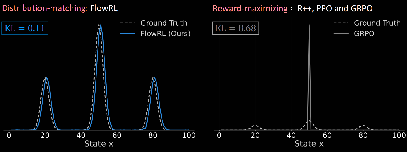
  • Most algorithms (eg, PPO or GRPO and its variants) aim purely to maximise rewards
  • FlowRL matches the policy to the full reward distribution
• Argues that this explicitly promotes diverse exploration and generalisable reasoning trajectories
• Pros: observed improvements for FlowRL vs PPO/GRPO/REINFORCE++:
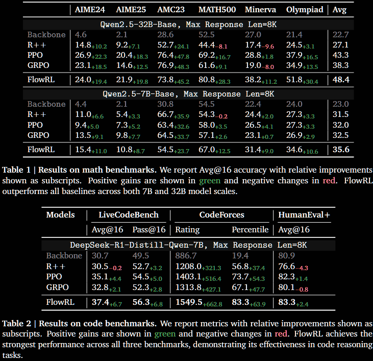
  • better scores on maths/code benchmarks
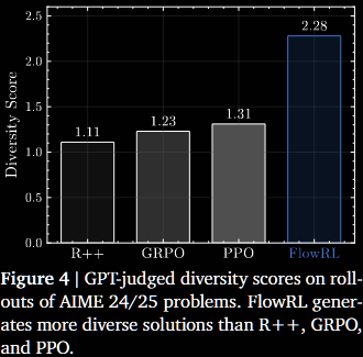
  • more diverse reasoning traces, sometimes significantly
• Cons: no comparison with more recent GRPO variants which also promote diversity
• Code is available on GitHub, based on verl: FlowRL

Elevator Pitch

Mainstream reasoning LLMs are trained with reward-maximising RL methods. These tend to overfit to the dominant reward signal, neglecting all other reasoning paths—model collapse. Such other paths have a lower reward, but may still be valid—eg, simply longer or less elegant. FlowRL aims to minimise the (reverse) KL divergence between the LLM's policy $\pi_\theta(y \mid x)$ and a target distribution $\propto e^{\beta r(x, y)}$, where $r(x, y)$ is the reward for answering $y$ to question $x$.

The evaluation focusses on maths/code benchmarks and LLM-judged diversity of responses. Improvements in both are observed vs GRPO and PPO. However, it must be noted that there are many variants of GRPO explicitly designed to address diversity issues, such as DAPO, ProRL or GSPO/GMPO.

Methodology

Reward Maximisation to Distribution Matching

The objective is to minimise a (reverse) KL divergence between the LLM's policy and a target distribution. Inspired by energy-based modelling, which comes from statistical physics, the target is a Gibbs measure given question $x$:

$e^{\beta r(x, y)} / Z(x)$, where $r(x, y)$ is the reward, $\beta$ the inverse temperature and $Z(x)$ the partition function.

As always, the partition function is intractable; it is thus parametrised ($Z = Z_\phi$) and learned. The objective is then to minimise

$$\min_\theta \mathbb E_{X \sim q}\bigl[ \mathsf{KL}\bigl( \pi_\theta(\cdot \mid X) \mathrel{\|} e^{\beta r(x, y)} / Z_\phi(x) \bigl) \bigr], \tag{$\star$}$$

where $q$ is a distribution over potential questions. (The expectation over $x$ is my assumption: it is not explained in the paper.)

This KL objective is approached via the framework of GFlowNets.

GFlowNets: brief summary.

Paraphrasing §2, GFlowNets are a probabilistic framework for training stochastic policies to sample discrete, compositional objects (eg, graphs or sequences) in proportion to a given reward. The core principle is to balance forward and backward probability flows at each state, inspired by flow matching (Bengio et al, 2021).

The technical observation (not knew to FlowRL) is that, in terms of expected gradients, minimising the KL objective in $(\star)$ is equivalent to minimising the trajectory balance (TB) loss in GFlowNets. It is stated informally and non-rigorously in the FlowRL paper.

Proposition 1 (informal). In terms of expected gradients, minimising the KL objective in $(\star)$ is equivalent to minimising the TB loss used in GFlowNet: $$\min_\theta \underbrace{ \mathsf{KL}\bigl( \pi_\theta(y \mid x) \mathrel{\|} e^{\beta r(x, y)} / Z_\phi(x) \bigl) }_{\text{standard KL divergence}} \iff \min_\theta \underbrace{ \bigl( \log Z_\phi(x) + \log \pi_\theta(y \mid x) - \beta r(x, y) \bigr)^2 }_{\text{trajectory balance in GFlowNets}}$$

Formally, this should be interpreted in the following way.

Proposition 1 (formal). For a question $x$ and response $y$, denote the pointwise KL and TB losses as follows: $$\begin{aligned} \mathcal L^\mathsf{KL}_\theta(x) &:= \mathsf{KL}\bigl( \pi_\theta(\cdot \mid x) \mathrel{\|} e^{\beta r(x, \cdot)} / Z(x) \bigr); \\ \mathcal L^\mathsf{TB}_{\theta, \phi}(x, y) &:= \bigl( \log \pi_\theta(y \mid x) + \log Z_\phi(x) - \beta r(x, y) \bigr)^2. \end{aligned}$$ Then, the "expected TB gradient" equals the (full) KL gradient: $$2 \nabla_\theta \mathcal L^\mathsf{KL}_\theta(x) = \mathbb E_{Y \sim \pi_\theta(\cdot \mid x)}[\nabla_\theta \mathcal L^\mathsf{TB}_{\theta, \phi}(x, y)].$$ In other words, to get an unbiased estimator of $\mathcal L^\mathsf{KL}_\theta(x)$, sample $Y \sim \pi_\theta(\cdot \mid x)$ and compute $\nabla_\theta \mathcal L^\mathsf{TB}_{\theta, \phi}(x, Y)$.

Derivation of formal version of Proposition 1.

Define the KL and trajectory balance (TB) objectives (losses), pointwise wrt questions $x$: $$\begin{aligned} \mathcal L^\mathsf{KL}_\theta(x) &:= \mathsf{KL}\bigl( \pi_\theta(\cdot \mid x) \mathrel{\|} e^{\beta r(x, \cdot)} / Z(x) \bigr); \\ \mathcal L^\mathsf{TB}_{\theta, \phi}(x, y) &:= \bigl( \log \pi_\theta(y \mid x) + \log Z_\phi(x) - \beta r(x, y) \bigr)^2. \end{aligned}$$ Expanding the KL divergence, $$\begin{aligned} \mathcal L^\mathsf{KL}_\theta(x) &= \mathbb E_{Y \sim \pi_\theta(\cdot \mid x)}\bigl[ \log\bigl( \pi_\theta(Y \mid x) Z(x) / e^{\beta r(x, Y)} \bigr) \bigr] \\ &= \mathbb E_{Y \sim \pi_\theta(\cdot \mid x)}\bigl[ \log \pi_\theta(Y \mid x) + \log Z(x) - \beta r(x, Y) \bigr]. \end{aligned}$$

The law of $Y \sim \pi_\theta(\cdot \mid x)$ depends on the parameters $\theta$. Abbreviate $$\delta_\theta(x, y) := \log \pi_\theta(y \mid x) + \log Z(x) - \beta r(x, y),$$ which has $$\nabla_\theta \delta_\theta(x, y) = \nabla_\theta \log \pi_\theta(y \mid x).$$

Start with the KL term, using $\pi_\theta(y \mid x) \nabla_\theta \log \pi_\theta(y \mid x) = \nabla_\theta \pi_\theta(y \mid x)$ and $\sum_y \nabla_\theta \pi_\theta(y \mid x) = \nabla_\theta \sum_y \pi_\theta(y \mid x) = \nabla_\theta 1 = 0$: $$\begin{aligned} \nabla_\theta \mathcal L^\mathsf{KL}_\theta(x) &\textstyle = \sum_y \nabla_\theta \bigl( \pi_\theta(y \mid x) \delta_\theta(x, y) \bigr) \\&\textstyle = \sum_y \bigl( \nabla_\theta \pi_\theta(y \mid x) \cdot \delta_\theta(x, y) + \pi_\theta(y \mid x) \cdot \nabla_\theta \log \pi_\theta(y \mid x) \bigr) \\&\textstyle = \sum_y \nabla_\theta \pi_\theta(y \mid x) \cdot (\delta_\theta(x, y) + 1) \\&\textstyle = \sum_y \nabla_\theta \pi_\theta(y \mid x) \cdot \delta_\theta(x, y) \\&\textstyle = \mathbb E_{Y \sim \pi_\theta(\cdot \mid x)}\bigl[ \nabla_\theta \log \pi_\theta(Y \mid x) \cdot \delta_\theta(x, Y) \bigr]. \end{aligned}$$ This is the policy gradient form. Turning to the TB term, the derivative is taken before the expectation over $y$: $$\nabla_\theta \mathcal L^\mathsf{TB}_{\theta, \phi}(x, y) = \nabla_\theta \delta_\theta(x, y)^2 = 2 \nabla_\theta \log \pi_\theta(y \mid x) \cdot \delta_\theta(x, y).$$ Hence, $$\begin{aligned} 2 \nabla_\theta \mathcal L^\mathsf{KL}_\theta(x) & = 2 \nabla_\theta \mathbb E_{Y \sim \pi_\theta(\cdot \mid x)}[ \delta_\theta(x, Y) ] \\& = \mathbb E_{Y \sim \pi_\theta(\cdot \mid x)}[ 2 \nabla_\theta \log \pi_\theta(Y \mid x) \cdot \delta_\theta(x, Y) ] = \mathbb E_{Y \sim \pi_\theta(\cdot \mid x)}[ \nabla_\theta \mathcal L^\mathsf{TB}_{\theta, \phi}(x, Y) ]. \end{aligned}$$

This squared-loss approach has a key advantage over direct KL optimisation: $Z_\phi(x)$ can be treated as a learnable parameter, rather than requiring explicit computation of the intractable partition function $Z(x)$. Using a stable squared-loss form is also advantageous practically.

However, the actual value of $Z_\phi(x)$ has no effect on the expected gradients. Indeed, $$\nabla_\theta \mathcal L^\mathsf{TB}_{\theta, \phi}(x, y) = \nabla_\theta \log \pi_\theta(y \mid x) \cdot g(x, y; \theta) \quad\textsf{where}\quad g(x, y; \theta) := \log \pi_\theta(y \mid x) + \log Z_\phi(x) - \beta r(x, y).$$ But, $\mathbb E_{Y \sim \pi_\theta(\cdot \mid x)}[\nabla_\theta \log \pi_\theta(Y \mid x)] = 0$. Hence, adding anything to $g$ that is independent of $\theta$ does not affect $\mathbb E_{Y \sim \pi_\theta(\cdot \mid x)}[ \nabla_\theta \mathcal L^\mathsf{TB}_{\theta, \phi}(x, y) ].$

That doesn't mean that $Z_\phi(x)$ should be ignored. Rather, it plays the same role as the baseline in standard RL training. The true partition function minimises the variance.

Learning Z_φ: gradients and regression.

Looking back at the per-$x$ KL objective, define $$\mathcal L^\mathsf{KL}_{\theta, \phi} := \mathbb E_{Y \sim \pi_\theta(\cdot \mid x)}\bigl[ \log \pi_\theta(Y \mid x) + \log Z_\phi(x) - \beta r(x, Y) \bigr];$$ then, $\mathcal L^\mathsf{KL}_{\theta, \phi} = \mathcal L^\mathsf{KL}_\theta$ if $Z_\phi = Z$.In order to minimise the variance, $Z_\phi(x)$ should be such that $$\log Z_\phi(x) = \mathbb E_{Y \sim \pi_\theta(\cdot \mid x)}[ \beta r(x, Y) - \log \pi_\theta(Y \mid x) ] = \mathbb E_{Y \sim \pi_\theta(\cdot \mid x)}\bigl[ \log\bigl( e^{\beta r(x, Y)} / \pi_\theta(Y \mid x) \bigr) \bigr].$$ Interestingly, this is not the true partition function $Z(x)$: indeed, $$\log Z(x) = \log \mathbb E_{Y \sim \pi_\theta(\cdot \mid x)}\bigl[ e^{\beta r(x, Y)} / \pi_\theta(Y \mid x) \bigr].$$ Calculating either exactly is intractable, so least-squares regression is used: $$\textsf{minimise} \quad \bigl( \log Z_\phi(x) - \beta r(x, y) + \log \pi_\theta(y \mid x) \bigr)^2 = \mathcal L^\mathsf{TB}_{\theta, \phi}(x, y) \quad\textsf{wrt}\quad \phi.$$

Taking derivative wrt $\phi$, $$\nabla_\phi \mathcal L^\mathsf{TB}_{\theta, \phi} = 2 \bigl( \nabla_\phi \log Z_\phi(x) - \beta r(x, y) + \log \pi_\theta(y \mid x) \bigr).$$ Thus, the following update is used: sample $y_1, ..., y_N \sim^\mathsf{iid} \pi_\theta(\cdot \mid x)$ and replace $$\textstyle \log Z_\phi(x) \leftarrow (1 - \eta) \log Z_\phi(x) + \eta \cdot \frac1n \sum_{i=1}^N \bigl( \beta(r, y_i) - \log \pi_\theta(y_i \mid x) \bigr),$$ where $\eta \in (0, 1]$ is the learning rate.

Proposition 5 in Appendix B shows the optimisation problem in Proposition 1 is equivalent, in the same sense, to $$\max_\theta \big\{ \mathbb E_{Y \sim \pi_\theta(\cdot \mid x)}\bigl[ \beta r(x, y) - \log Z_\phi(x) \bigr] + \mathcal H\bigl( \pi_\theta(\cdot \mid x) \bigr) \big\},$$ where $\mathcal H(\mu) := - \mathbb E_{X \sim \mu}[\log \mu(X)]$ denotes the entropy of the distribution. So, the FlowRL objective can be interpreted as jointly maximising reward and entropy. This encourages the policy to cover the entire reward-weighted distribution, rather than collapsing to a few high-reward modes.

FlowRL

Proposition 1 is not new to FlowRL. However, its application to long context is new. Previous GFlowNets works typically operate on short trajectores in small, discrete spaces (no citation given). Long CoT reasoning introduces two challenges.

1. Exploding gradients. The log-probability term $\log \pi_\theta(y \mid x)$ decomposes as $\sum_t \log \pi_\theta(y_t \mid y_{< t}, x)$, causing the gradient to potentially scale with sequence length.

2. Sampling mismatch. Mainstream RL algorithms often perform micro-batch updates and reuse trajectories collected from an old policy, for efficiency reasons. Contrastingly, the KL-based trajectory balance (TB) objective assumes fully on-policy sampling, with responses drawn from the current policy.

Neither of these issues is new to RL post-training of LLMs. Exploding gradients are addressed by length normalisation, rescaling as $$\tfrac1{|y|} \log \pi_\theta(y \mid x) = \log \pi_\theta(y \mid x)^{1/|y|}.$$ The sampling mismatch is handled with importance sampling in a relatively standard way, alongside some clipping: $$w = \operatorname{clip}\bigl( \pi_\theta(y \mid x) / \pi_{\theta_\mathsf{old}}(y \mid x), 1 - \varepsilon, 1 + \varepsilon \bigr)_\textsf{detach},$$ where the subscript-"detatch" indactes that the gradient is detatched during its calculation.

Following established practices in the GFlowNets literature, a reference model is incorporated as a prior constraint on the reward distribution: $$e^{\beta r(x, y)} \quad\textsf{is replaced with}\quad e^{\beta r(x, y)} \cdot \pi_\textsf{ref}(y \mid x).$$ Naturally, $Z(x)$ should now be updated; although, as discussed above, its actual value doesn't affect the gradients, only the variance. This adjustment leads to the following minimisation problem: $$\min_\theta \bigl( \log Z_\phi(x) + \log \pi_\theta(y \mid x) - \beta r(x, y) - \log \pi_\mathsf{ref}(y \mid x) \bigr).$$

Additionally, as in GRPO, group normalisation is applied to $r(x, y)$: $$\hat r_i = (r_i - \operatorname{mean} r) / \operatorname{std} r,$$ where $r = \{r_1, ..., r_G\}$ denotes a set of rewards within a sampled group.

Substituting all this into Proposition 1 provides the following objective: $$\mathcal L^\mathsf{FlowRL}_{\theta, \phi}(x, y) := w \bigl( \log Z_\phi(x) + \tfrac1{|y|} \log \pi_\theta(y \mid x) - \beta \hat r_i(x, y) - \tfrac1{|y|} \log \pi_\mathsf{ref}(y \mid x) \bigr)^2.$$

Results

FlowRL is compared with fairly 'vanilla' RL algorithms: REINFORCE++ (2025/01), PPO (2017/07) and GRPO (2024/12). There are modern variants, or tweaks, of GRPO which explicitly address diversity, such as DAPO (2025/03) or ProRL (2025/05). Others, such as GSPO (2025/07) and GMPO (2025/07), address stability. It is highly disappointing that no comparison with these is done—especially as multiple are mentioned in the paper. At least relatively large models are used: 7B and 32B.

Nevertheless, the reported results are included below, for completeness.