Soft Thinking Summary

Soft Thinking: Unlocking the Reasoning Potential of LLMs in Continuous Concept Space

• 2025-05; Zhang, He, Yan, Shen, Zhao, Wang, Shen, Wang

High-Level Ideas

• Training-free method that enables human-like 'soft' reasoning
• Standard Chain-of-Thought (CoT) sample one token per step and follow that path, potentially abandoning valuable alternatives
• Soft Thinking generates concept tokens in continuous concept space corresponding to LLM-produced distribution over the vocab (at given step)
• It's related to superposition of all possible tokens: it's a convex combination, weighted by probabilities
• This flexibility enables the exploration of different reasoning paths, and avoids making hard (consequential) decisions too early
• A cold stop (entropy threshold) is used to mitigate out-of-distribution issues

Related Papers

• Let Models Speak Ciphers: Multiagent Debate through Embeddings

  • main idea (weighted average of embedded tokens) seems exactly the same
  • CIPHER paper also has a debate element

• Text Generation Beyond Discrete Token Sampling ("Mixture of Inputs")

  • Mixes the distribution (soft thinking) with the sampled token (CoT)
  • When only using distribution, calls it Direct Mixture; performs badly, but no cold stop

• Training Large Language Models to Reason in a Continuous Latent Space (COCONUT)

• Reasoning by Superposition: A Theoretical Perspective on Chain of Continuous Thought

Some Details

Instead of injecting the random, one-hot encoded token, after embedding, into the LLM, the concept token is injected back:

inject $\sum_{k=1}^{|V|} \mathsf{ct}[k] e(k)$

where $\mathsf{ct}[k]$/$e(k)$ is the selection probability/embedding of the $k$-th vocab item.

The theoretical justification is based on linear approximations in the expression

$$\textstyle p(y \mid x) = \sum_{t_1} p(t_1 \mid x) \sum_{t_2} p(t_2 \mid x, t_1) ... \sum_{t_m} p(t_m \mid x, t_{1:m-1}) p(y \mid x, t_{1:m});$$

here, $t_j$ is the $j$-th (intermediate reasoning) token. To emphasise, $p(\cdot \mid x, t_{1:j})$ is the probability of the next token given the input $x$ and intermediate reasoning tokens $t_1, ..., t_j$. Once some stopping criterion is achieved, the model outputs an answer, denoted $y$.

This expansion entails exponentially-in-$m$ many paths, indexed by the choice of intermediate reasoning tokens. If we only expanded one layer,

$$\textstyle p(y \mid x) = \sum_{t_1} p(t_1 \mid x) p(y \mid x, t_1).$$

In expectation,

$$\textstyle \mathsf{ct}_1 = \mathbb E[t_1] = \sum_{t_1} p(t_1 \mid x) t_1 = p(\cdot \mid x)/$$

Linearising the previous expression about its mean, (ie, replacing random $t_1$ by its non-random mean $\mathsf{ct}_1$),

$$\textstyle p(y \mid x) = \sum_{t_1} p(t_1 \mid x) p(y \mid x, t_1) \approx p(y \mid x, \sum_{t_1} p(t_1 \mid x) t_1) = p(y \mid x, \mathsf{ct}_1).$$

The approximation is repeated given $\mathsf{ct}_1$:

$$\textstyle p(y \mid x, \mathsf{ct}_1) = \sum_{t_2} p(t_2 \mid \mathsf{ct}_1) p(y \mid x, \mathsf{ct}_1, \mathsf{ct}_2) \approx p(y \mid x, \mathsf{ct}_1, \mathsf{ct}_2).$$

Iterating,

$$p(y \mid x) \approx p(y \mid x, \mathsf{ct}_1, \mathsf{ct}_2, ..., \mathsf{ct}_m).$$

In contrast, discrete CoT replaces each summation $\sum_{t_j} p(t_j \mid \cdot)$ with sampling a single token, which discards the mass from all other paths. Soft thinking preserves the distribution through the concept tokens, whilst collapsing the exponential path summation to a single forward pass.

A cold stop is also implemented, where the entropy is tracked in real time. This is to address issues in which the continuous concept tokens place the model in an out-of-distribution regime. If the entropy (ie, uncertainty) of a concept token drops below a threshold, the process stops. A basic ablation study is conducted; with details below.

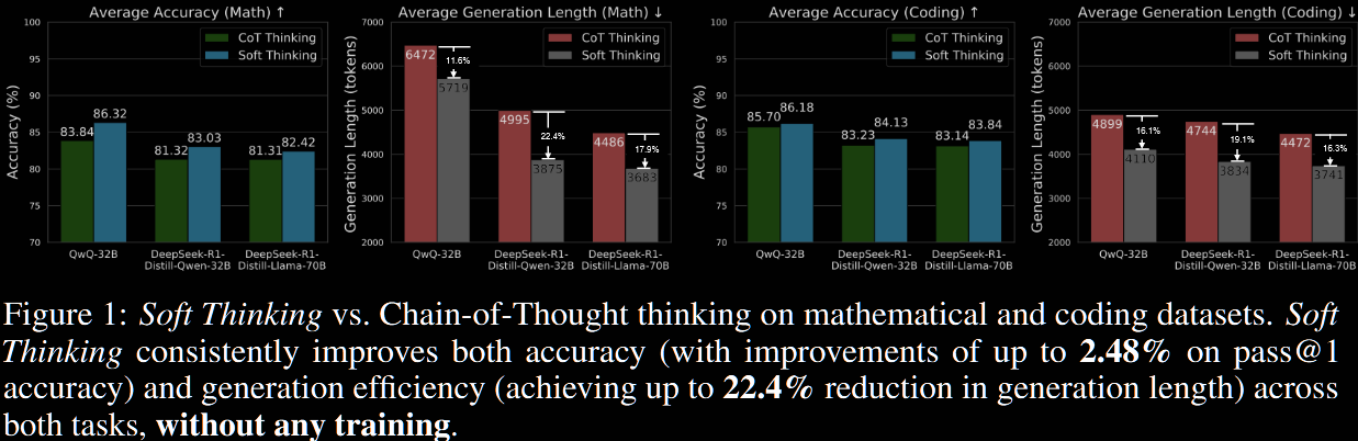
Results

In summary, I'd suggest that the accuracy increase is modest, but the generation length reduction is significant.

The first table is the accuracy (higher → better) and the second the generation length (lower → better).

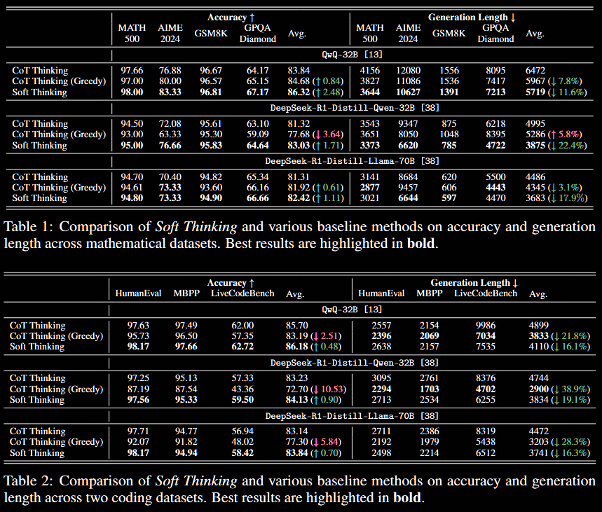
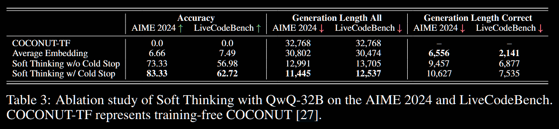
The soft thinking results all utilise a cold stop, with threshold $\tau$ optimised for the problem at hand. An ablation study is conducted regarding cold stop—namely, $\tau = 0$ is forced, ensuring the cold stop is never activated.

The four lines in the table below correspond to different strategies.

• COCONUT-TF: the training-free COCONUT approach simply feeds the previous hidden state as the next input embedding.

• Average Embedding: the (embeddings of the) top 5 tokens are averaged and fed.

• w/o Cold Stop: soft thinking without cold stop—ie, $\tau = 0$ enforced.

• w/ Cold Stop: full soft thinking, with cold-stop threshold $\tau$ optimised (swept).

This is all summarised in a figure given above the abstract.