Magistral Summary

• Magistral
• 2025-06; Magistral-AI

High-Level Summary

• Introduces Magistral, a reasoning model (Medium and Small)
• Ground-up approach, relying on Minstral models and infrastructure
• Adjusts and uses GRPO
• Detailed description of training methods, good to learn from

Methodology

This section describes the fundamental RL methodology. It is based on GRPO, but adapted and adjusted.

GRPO Adaptation

Vanilla GRPO optimises the expectation over $q \sim P(Q)$ and $o_1, ..., o_G \sim^\mathsf{iid} \pi_{\theta_\text{old}}(\cdot \mid q)$ of

$$\frac1G \sum_{i=1}^G \frac1{|o_i|} \sum_{t=1}^{|o_i|} \biggl( \operatorname{min–clip}_\varepsilon\biggl( \frac{\pi_\theta(o_{i,t} \mid q, o_{i, < t})}{\pi_{\theta_\text{old}}(o_{i, t} \mid q, o_{i, < t})} \widehat A_{i, t} \biggr) - \beta \operatorname{KL}\bigl( \pi_\theta(\cdot \mid q) \mathrel{\|} \pi_\text{ref}(\cdot \mid q) \bigr) \biggr),$$

where $q$ represents the query, $o$ the generated output and $\pi_\text{ref}$ a reference model; the relative advantage, or group normalised advantage, is given by

$$\widehat A_{i, t} = \frac{r_i - \operatorname{mean}(r_1, ..., r_G)}{\operatorname{std}(r_1, ..., r_G)},$$

where $r_1, ..., r_G$ are the rewards corresponding to generations (outputs) $o_1, ..., o_G$.

Minstral introduce several modifications (collapsible sections).

1. Eliminating KL divergence.

   The KL penalty constrains the online policy from ever deviating too far from the initial model. In practice, they found that the policy diverged substantially regardless, and so discarded this term altogether (set $\beta = 0$). This also removes the need to store a copy of the reference model.

   Personally, I always found this KL term odd: it restricts the policy from deviating from the reference, rather than restricting an update (vs the current).

2. Loss normalisation.

   Long sequences with few 'turning points'—ie, places where the policy ratio is not close to $1$—get significantly down-weighted by their large $|o_i|$. The normalisation

   $$\textstyle G^{-1} \sum_{i=1}^G |o_i|^{-1} \sum_{t=1}^{|o_i|} (...) \quad\text{is replaced with}\quad (\sum_{i=1}^G |o_i|)^{-1} \sum_{i=1}^G \sum_{t=1}^{|o_i|} (...).$$

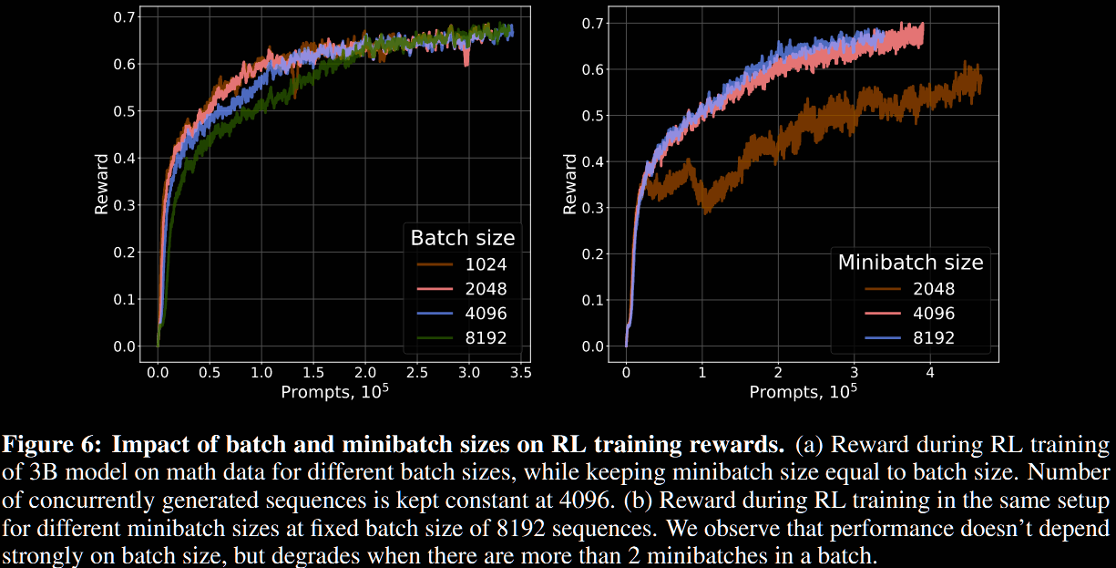
   This is no change if $|o_i|$ is a fixed length. No ablation study is conducted on this aspect directly, but there is one on batch/minibatch sizes.

3. Advantage normalisation.

   The advantage is always centred wrt the question: $\widetilde A_i = r_i - \operatorname{mean}(r_1, ..., r_G)$, where $r_1, ..., r_G$ are the rewards received in the $G$ answers to the same question. The rewards are then normalised wrt the standard deviations of the advantages $\widetilde A_i$ in a minibatch, to get the final estimate $\widehat A_i = \widetilde A_i / \operatorname{std}((\widetilde A_i)_{i \in B})$, where $B$ is a minibatch.

   The idea is that easy/hard questions with low standard deviations get up-weighted in the original GRPO. However, an ablation study in §6.4 suggests this has little effect over the usual version.

4. Relaxing trust region.

   Standard GRPO clipping $\varepsilon \approx 0.2$ limits exploration by restricting the increase in probability of low-likelihood tokens. Minstral allow the model to explore rare steps by following the clip-higher strategy: the upper threshold is replaced with a larger $\varepsilon_\text{high} \in [0.26, 0.28]$, with the lower $1\varepsilon_\text{low} \approx 0.2$ roughly unchanged.

5. Eliminating non-diverse groups.

   Groups where all generations are wrong/right contribute nothing, so are removed. Presumably, this is done in the original GRPO too, with the convention $\widehat A_i = (0 - 0)/0 := 0$ (ie, no advantage).

Reward

Choosing the reward is one of the most impactful aspects of an RL algorithm. They focus on four aspects.

1. Formatting: +0.1/+0.

   For maths and code problems, a specific format is imposed. Failure to meet any of these conditions sets the reward to $0$, and no further grading is undertaken. Otherwise, a reward of $0.1$ is granted, and grading proceeds.

2. Correctness: +0.9/+0.

   A correct answer (after some equivalence and runtime considerations) is granted an additional $0.9$, taking the total to $1$.

3. Length penalty: up to -0.9.

   If the length exceeds $\ell_\text{cache}$, a linear penalty is applied, up to $-0.1$ at $\ell_\text{max}$.

4. Language consistency: +0.1/+0.

   An additional $+0.1$ is granted if the response is in the same language is used for the whole conversation—ie, the model follows the user's language.

They found that the RL training was sensitive to the system prompt: eg, including "be as casual and as long as you want" in the prompt increased the entropy, and hence exploration, of the model.

Infrastructure

Significant details around their infrastructure, and how they overcame difficulties in distributed RL, are given. It is not repeated here, but is worth bearing in mind for future implementations. The details are in §3, and are only about one page of text plus a couple of figures.

Data Curation

The problems are limited to those with verifiable solutions: maths with numerical answers or expression and coding with associate tests. They focus on the particulars of their maths and code evaluation, but include a key difficulty filtering insight.

A two-stage filtering pipeline is implemented to create 'Goldilocks' difficulty-level questions: neither too easy nor too hard for the model to learn from.

1. • Perform initial difficulty assessment using Mistral Large 2 (not a reasoning model): sample 16 responses, and remove those never/always solved.
   • Use this curated set to train a 24B model via RL pipeline, resulting in a small but fairly good checkpoint used solely for difficulty assessment.
2. • This stronger RL-trained model re-assesses the entire dataset: again, sample 16 responses, filtering out the easiest/still-unsolved problems.
   • Further filter out potentially incorrect problems, where a majority of samples have the same final answer but disagree with the "ground-truth".

The authors argue that this two-stage methodology was crucial, that a single pass with the weaker Mistral Large 2 model would've caused it to discard difficult, but possible, questions, incorrectly classifying them as unsolvable

Experiments and Results

The primary goal is to answer two questions.

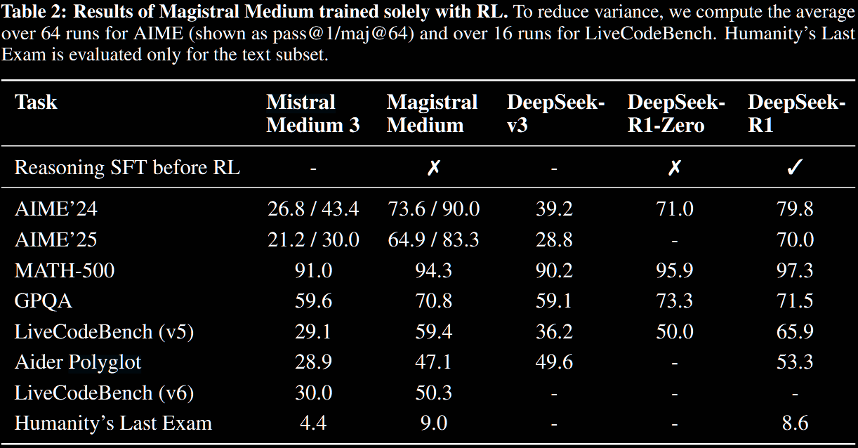
1. How far can one get with pure RL on a large base model?
2. Given a strong teacher model, how can one achieve the strongest possible lightweight model?

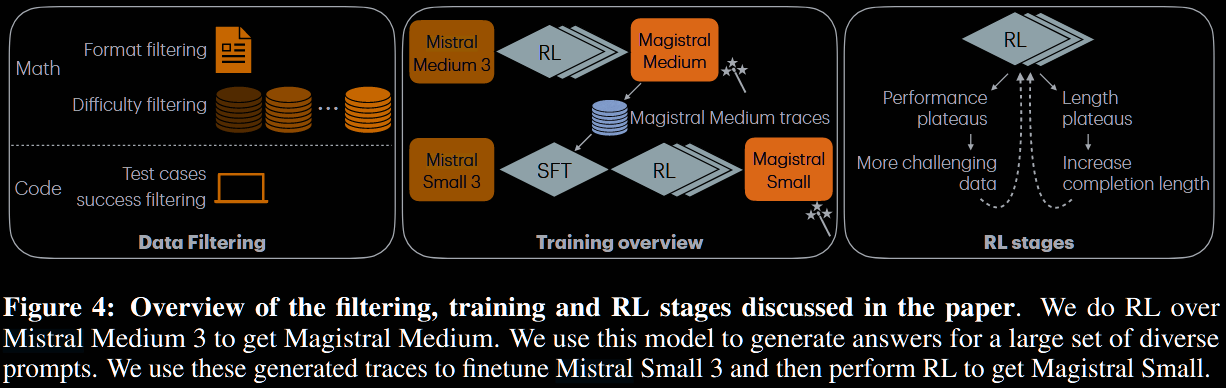
TO this end, Magistral Medium is trained on top of Mistral Medium 3 with pure RL, and Magistral began with SFT traces derived from Magistral Medium.

Magistral Medium: Reasoning RL from Scratch

Training was done in multiple stages, with distinct hyperparameters, ensuring the following criteria hold.

1. Dataset isn't too easy.

   Increase the difficulty (as judged previously) as model performance increases. Data previously filtered out for being too difficult can be added, and completely solved problems removed.

   It may be worth updating estimate on the difficulty as the model improves: if it continually can't solve something, maybe defer it until later.

2. Generation length doesn't stop growing.

   Both maximal allowed length $\ell_\text{max}$ and unpunished length $\ell_\text{max} - \ell_\text{cache}$ are increased over time to prevent stagnation.

3. KV-cache memory burden is not too large.

   As generation length increases, so does memory associated with KV cache. The total number of concurrent requests, batch size and minibatch size are decreased during training.

Magistral Small: RL on Top of Reasoning SFT Bootstrapping

The next objective is to train a strong student model (Magistral Small) given a strong teacher (Magistral Medium).

Magistral Small is 'cold-started' with SFT traces from Magistral Medium. The general feeling is that pure RL training benefits from a small set of extremely clean and difficult training points. Contrastingly, diversity of prompts was found to be important for the reasoning cold.

1. Begin by extracting traces with correct answers from the RL training of Magistral Medium, excluding those from early steps with short CoTs. Maintain a mixed difficulty level.

2. Augment this SFT cold-start data by generating responses from Magistral medium on a large set of diverse prompts, with mixed difficulty.

3. Train this SFT checkpoint with RL, with temperature $1.0$ (vs $0.7$ used for Magistral Medium) and encourage exploration via $\varepsilon_\text{high} = 0.3$ (vs $\varepsilon \approx 0.25$ before).

Ablation Studies.

Some ablation studies are given in §6. They are very briefly summarised here.

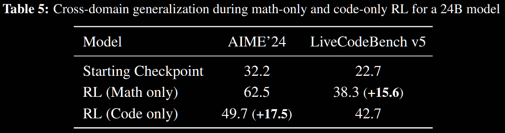
1. Cross-domain generalisation.

   Two RL experiments on the 24B model are conducted: one where the model is trained exclusively on maths data and the other exclusively on code; both are evaluated on all data. The table below demonstrates strong performance on out-of-domain tasks.

   

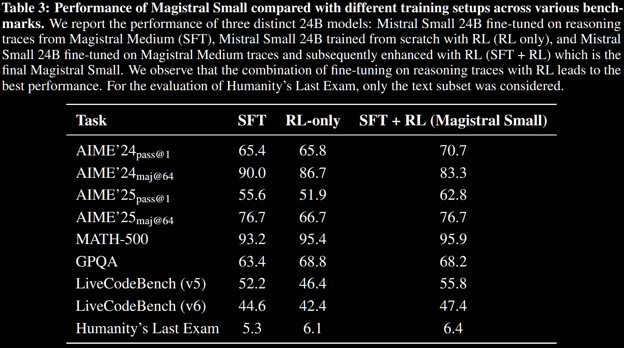
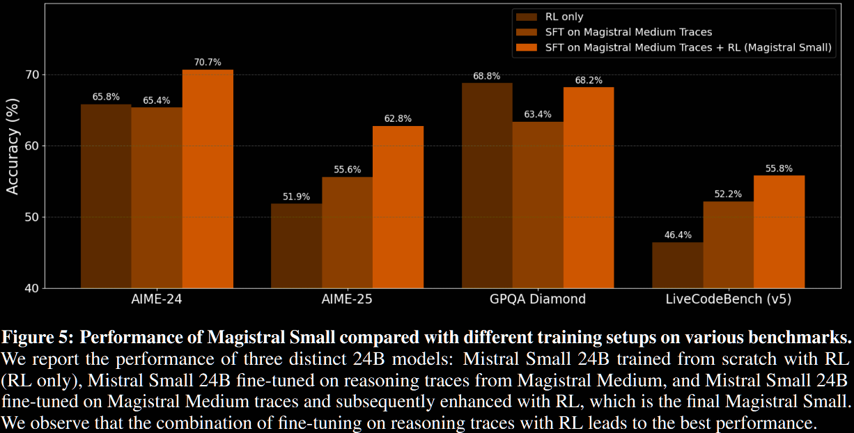
2. Distillation vs RL for small models

   Previous work observed that smaller models relying solely on RL did not perform well compared with those distilled from larger reasoning models. This doesn't appear here; eg, Mistral Small 3 + pure RL achieves similar performance on AIME'24 as the distilled version, outperforming on MATH and GPQA and only slightly worse on code benchmarks.

   

3. Batch and minibatch sizes

   Different scales are considered. See §6.3 for details.

   

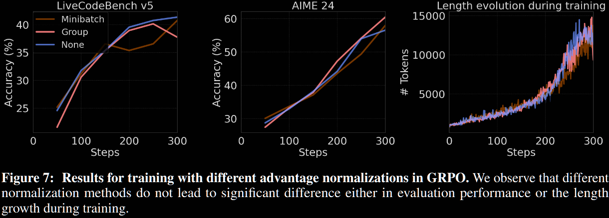
4. Advantage normalisation.

   Three advantage strategies were experimented with.

   1. Minibatch: normalise advantages within a minibatch (as described previously)
   2. Group: normalise advantages within a group over a single prompt (as in vanilla GRP)
   3. No normalisation: do not normalise

   Previous work noted that normalisation over groups can bias easy/hard questions, due to their lower standard deviation. No significant effect was observed here. As a result, minibatch normalisation was chosen (for convenience?) for the main experiments.

   

Further Analysis

A deep-dive into the dynamics of RL training, leading to evidence that increasing the completion length is the primary aspect that improves performance, is given in §7. Additionally, two methods that didn't work are outlined:

• giving more fine-grained rewards in code tasks based on test completion rate;
• controlling entropy via a bonus term in the loss—even though this is a common strategy.

We do not repeat this section here.